Multimodal Tokenization with Vector Quantization: A Review

How do we bridge the gap between continuous perceptual signals and the discrete token sequences that autoregressive models excel at? This question sits at the heart of modern multimodal AI. Vector quantization (VQ)¹ offers an elegant answer: learn a finite codebook that compresses high-dimensional inputs—images, audio, video—into compact discrete codes, enabling unified sequence modeling across modalities.

Over the past few years, the design of VQ-based tokenizers has quietly become one of the most consequential architectural choices in large multimodal models. The quality of the learned codebook directly determines the information bottleneck: too small and you lose fidelity; too large and the prior becomes intractable. This tension has driven a rich line of work—from VQ-VAE’s straight-through estimator, to VQGAN’s perceptual-adversarial training, to more recent lookup-free methods (LFQ, FSQ, BSQ) that sidestep codebook collapse entirely.

This post traces that evolution systematically: we start from the foundational VQ-VAE formulation, walk through residual and hierarchical quantization schemes (RQ-VAE, HQ-VAE), examine how generation architectures (autoregressive transformers, masked prediction) consume these tokens, and survey the latest simplifications that make VQ practical at scale. The goal is not just a catalog of methods, but a coherent picture of why each design choice was made and what trade-offs it introduces.

Codebook Learning with Vector Quantization

VQ-VAE (NeurIPS’17)

Vector-Quantized AutoEncoder (VQ-VAE)² combines variational autoencoders (VAE) with vector quantization (VQ)¹, parameterizing the posterior distribution of discrete latents given an observation.

Note: It does not suffer from large variance, and avoids the ‘‘posterior collapse’’ issue which has been problematic with many VAEs that have a strong decoder, often caused by latents being ignored.

VAE

VAEs consist of three components: (1) an encoder parameterized by a posterior distribution $q(z\vert x)$ of discrete latent random variables $z$ given input $x$, (2) a prior distribution $p(z)$, and (3) a decoder with distribution $p(x\vert z)$ over input data.

Discrete latents

VQ-VAE defines the posterior and prior distributions as categorical, and the samples drawn from these distributions index an embedding table, which are used as the decoder inputs.

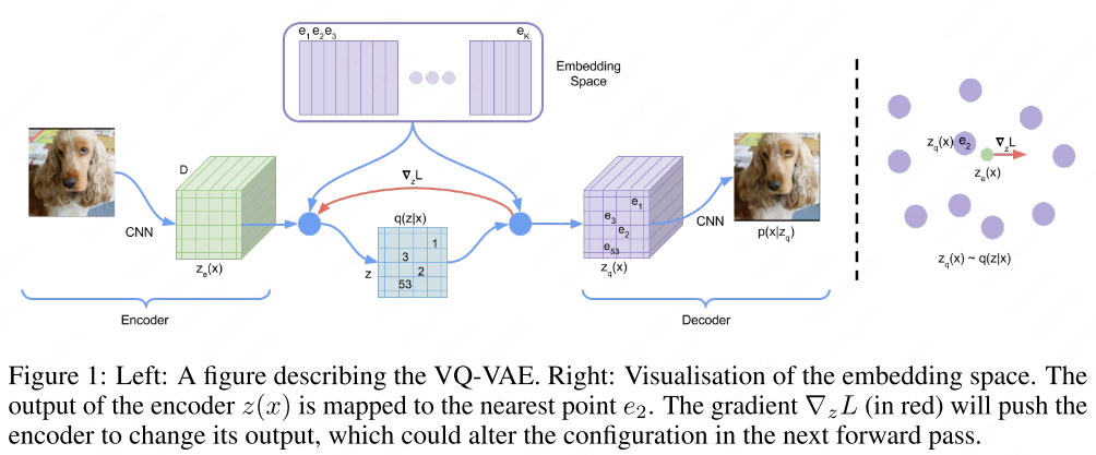
VQ-VAE defines the latent embedding space $e \in \mathbb{R}^{K \times D}$ where $K$ is the codebook size and $D$ is the embedding dimension, with \(e_i \in \mathbb{R}^D\) for $i \in {1,2,\cdots, K}$. The encoder maps input $x$ to output \(z_e(x)\), and the discrete latent $z$ is obtained via nearest-neighbor lookup in the shared embedding space $e$. The posterior categorical distribution $q(z\vert x)$ is defined as a one-hot distribution:

This can be viewed as a VAE where $\log p(x)$ is bounded by the ELBO. Since $q(z=k\vert x)$ is deterministic and the prior over $z$ is uniform, the KL divergence is constant and equals $\log K$.

The encoder output \(z_e(x)\) is passed through the discretization bottleneck and mapped to the nearest embedding vector \(e_k\), which serves as the decoder input:

This can be treated as an autoencoder with a particular non-linearity that maps the latents to 1-of-$K$ embedding vectors.

Training

Since Eq.$\eqref{eq:emb}$ and $\eqref{eq:posterior}$ involve non-differentiable operations, the gradient is approximated using the straight-through estimator (STE), which copies gradients from the decoder input \(z_q(x)\) directly to the encoder output \(z_e(x)\).

Here, $\beta=0.25$.

EMA Update

VQVAE can use exponential moving average (EMA) updates for the codebook, as the replacement for the codebook loss, the 2nd term in Eq.\(\eqref{eq:vq_loss}\).

where \(n_{i}^{(t)}\) is the number of quantized vectors in $E(x)$, $\gamma \in [0,1] $ is a decay parameter.

1
2
3
4
5
6
7
8
9
10
11
12
13
 
# reconstruction loss
loss = F.mse_loss(quantize, x.detach())
# determine code to use for commitment loss
maybe_detach = torch.detach if not self.learnable_codebook or freeze_codebook else identity

commit_quantize = maybe_detach(quantize)

# straight through
quantize = x + (quantize - x).detach()

commit_loss = F.mse_loss(commit_quantize, x)

loss = loss + commit_loss * self.commitment_weight
 

VQVAE-2 (NeurIPS’19)

VQ-VAE-2³ introduces a multi-scale hierarchical structure to the original VQ-VAE framework, complemented by PixelCNN priors that govern the latent codes.

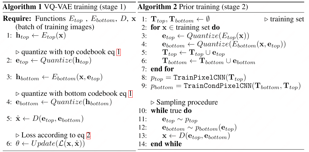
Stage 1: Hierarchical Latent Codes

Note: Motivation: Hierarchical VQ models capture local features, such as textures, distinctly from global features, like the shape and geometry of objects.

VQ-VAE-2³ employs a hierarchical arrangement of VQ codes to effectively model large images. In this hierarchy, the top-level latent code encapsulates global information, while the bottom-level latent code, which is conditioned on the top-level code, is tasked with capturing local details.

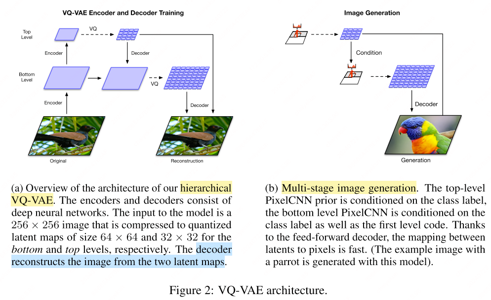
Without conditioning the bottom level on the top level, the top-level latent would need to encode every fine-grained pixel detail. By letting each level focus on different aspects (global structure vs. local texture), the hierarchy encourages complementary information across latent maps, reducing reconstruction error.

Stage 2: Learning Priors over Latent Codes

In the second stage, VQ-VAE-2 fits a prior distribution over the learned latent codes, effectively achieving lossless compression of the latent space. The authors find that incorporating self-attention layers helps capture long-range spatial correlations in the image.

VQGAN (CVPR’21)

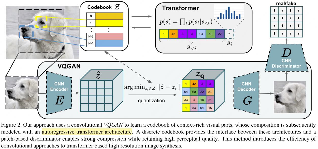
VQGAN⁴ combines CNNs with transformer architectures to learn a codebook of contextually rich visual elements. The transformer captures long-range interactions within global compositions, while an adversarial training strategy ensures the codebook captures perceptually significant local structures—reducing the transformer’s burden of modeling low-level statistics.

VQGAN employs a discriminator and perceptual loss to maintain high perceptual quality even at increased compression rates. It utilizes a patch-based discriminator $D$, trained to differentiate between real and reconstructed images:

Here, $E$ denotes the encoder, $G$ is the generator, and \(\mathcal{Z} = \{z_{k}\}_{k=1}^{K} \subset \mathbb{R}^{n_{z}}\) represents the learned discrete codebook.

The optimization objective for VQGAN is formulated as a min-max problem:

The adaptive weight $\lambda$ is computed as follows:

where \(\mathcal{L}_{\mathrm{recon}}\) is the perceptual reconstruction loss and \(\nabla_{G_L}[\cdot]\) denotes the gradient with respect to the last layer of the decoder.

In the second stage, VQGAN pretrains a transformer to predict rasterized image tokens autoregressively.

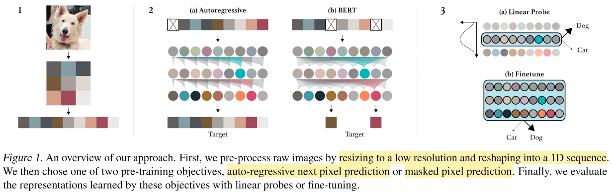
iGPT (ICML’20)

iGPT⁵ applies autoregressive pre-training directly to image pixels. It first reduces image resolution, then applies $k$-means clustering ($k=512$) to (R, G, B) pixel values, condensing the color space and reducing context length by $3\times$. For larger images, a VQ-VAE further compresses the pixel space into a $48^2$ latent grid.

Representation quality is evaluated via:

1. Linear probe: training a linear classifier on frozen pre-trained features.
2. Finetuning: end-to-end adaptation on downstream tasks.

DALL-E (ICML’21)

DALL-E⁶ applies a transformer that autoregressively models the text and image tokens as a single stream of data. It uses two-stage training procedure:

1. Stage 1: Train a discrete VAE to compress each $256 \times 256$ RGB image into a $32 \times 32$ grid of image tokens, each element of which can assume 8192 possible values.
2. Stage 2: Concatenate up to 256 BPE-encoded text tokens with the $1024 (32 \times 32)$ image tokens, and train an autoregressive transformer to model the joint distribution over the text and image tokens.

The overall procedure can be viewed as maximizing the evidence lower bound (ELBO) on the joint likelihood of the model distribution over images $x$, captions $y$, and the tokens $z$ for the encoded RGB image. We model this distribution using the factorization \(p_{\theta,\psi}(x,y,z)=p_{\theta}(x\mid y,z)p_{\psi}(y,z)\), which yields the lower bound:

where:

• \(q_\phi\) denotes the distribution over the $32\times 32$ image tokens generated by the dVAE encoder given the RGB image $x$;
• \(p_\theta\) denotes the distribution over the RGB images generated by the dVAE decoder given the image tokens;
• \(p_\phi\) denotes the joint distribution over the text image tokens modeled by transformer.

Stage 1: Visual Codebook Learning

DALL-E first trains a dVAE using Gumbel-Softmax relaxation instead of the straight-through estimator used in VQ-VAE. Each $256 \times 256$ RGB image is transformed into a $32 \times 32$ grid of discrete tokens through a discrete Variational Autoencoder (dVAE). These tokens can each take on one of 8192 unique values, resulting in a compact encoding of the visual information.

The dVAE leverages a Gumbel-Softmax relaxation technique, as opposed to the straight-through estimator often used in VQ-VAE. Its architecture comprises convolutional ResNets with bottleneck-style blocks, utilizing 3x3 convolutions and 1x1 convolutions for skip connections. Downscaling of feature maps is performed by max-pooling in the encoder, while the decoder employs nearest-neighbor upsampling for reconstruction.

Stage 2: Prior Learning

The subsequent stage is focused on modeling the relationship between text and images: The model concatenates up to 256 BPE-encoded text tokens with the 1024 image tokens from Stage 1. An autoregressive transformer is then trained to capture the joint distribution of both text and image tokens.

DALL-E normalizes the cross-entropy losses for text and image tokens by their respective totals in the data batch. The text token loss is weighted by $1/8$, and the image token loss by $7/8$, reflecting a higher emphasis on image modeling.

ViT-VQGAN (ICLR’22)

ViT-VQGAN⁷ leverages a ViT-based VQGAN to encode discrete latent codes, combining logit-laplace loss, L2 loss, adversarial loss, and perceptual loss.

ViT-VQGAN⁷ uses a combination of logit-laplace loss, L2 loss, perceptual loss based on VGG net, and GAN loss with a StyleGAN discriminator:

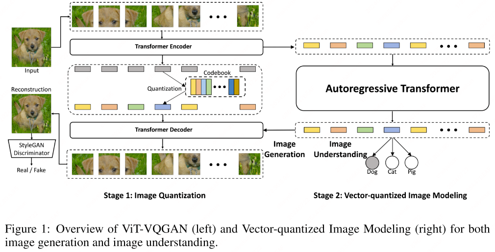
Dimension reduction: ViT-VQGAN⁷ finds that reducing the dimensionality of the lookup space significantly enhances reconstruction. By projecting from 256 to 32 dimensions via a linear mapping after the encoder, the model achieves more efficient and accurate reconstruction.

L2-normalized codes: L2 normalization is applied to both encoded latents \(z_e(x)\) and codebook latents $e$ (initialized from a normal distribution). This projects all latent variables onto a hypersphere, effectively turning Euclidean distance into cosine similarity: \(\Vert\ell_2(z_e(x))-\ell_2(e_j)\Vert_2^2\). Cosine similarity provides a more stable comparison in high-dimensional spaces where Euclidean distances can become inflated.

RQ-VAE (CVPR’22)

The Residual-Quantized Variational Autoencoder (RQ-VAE)⁸ incorporates residual quantization (RQ) to progressively refine the quantization of a feature map in a hierarchical, coarse-to-fine approach. At each quantized position, RQ-VAE employs a sequence of $D$ residual quantization iterations, yielding $D$ discrete codes. RQ’s ability to generate a vast number of compositions—exponential in the number of iterations ($D$)—allows RQ-VAE to closely approximate feature maps without depending on an excessively large codebook. This efficiency in representation enables a reduction in the spatial resolution of the quantized feature map without compromising the integrity of the encoded image.

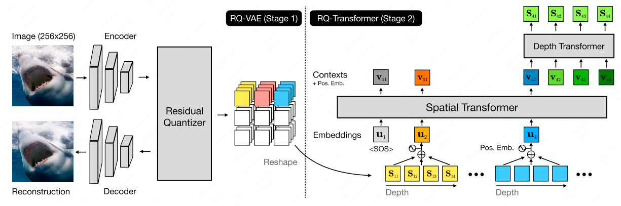
The dual-stage framework combines RQ-VAE with an RQ-Transformer, which is designed for the autoregressive modeling of images:

Stage 1: RQ-VAE encodes an image into a stacked map of $D$ discrete codes using a codebook. Stage 2: RQ-Transformer addresses the training challenges of autoregressive models, particularly exposure bias.

Stage 1: RQ-VAE

Note: Reducing Spatial Resolution: While VQ-VAE performs a form of lossy compression on images and necessitates a balance between dimensionality reduction and information preservation, it typically requires \(HW \log_2 K\) bits to encode an image using a codebook of size $K$. According to rate-distortion theory, the minimum reconstruction error is contingent on the bit count. To reduce spatial dimensions from $(H,W)$ to $(H/2,W/2)$ while maintaining reconstruction quality, the codebook would need to increase to a size of $K^4$. However, a VQ-VAE with an expansive codebook is impractical due to the potential for codebook collapse and unstable training dynamics.

Instead of enlarging the codebook, RQ-VAE applies residual quantization to discretize a vector $z$. Given a quantization depth $D$, RQ represents $z$ with a sequence of $D$ codes:

Here $\mathcal{C}$ is the codebook of size $\vert\mathcal{C}\vert=K$, and \(k_d\) is the code assigned to vector $z$ at depth $d$. Starting from the initial residual \(r_0 = z\), RQ iteratively computes the code \(k_d\) for the residual \(r_{d-1}\), and the subsequent residual \(r_d\) is determined as follows:

This process is repeated for $d=1,\cdots, D$.

While traditional VQ segments the entire vector space \(\mathbb{R}^{n_z}\) into $K$ distinct clusters, RQ with depth $D$ can partition this space into up to $K^D$ clusters. This gives RQ with depth $D$ a partitioning capacity comparable to VQ with $K^D$ codes.

RQ-VAE augments the encoder-decoder structure of VQ-VAE by replacing VQ with the RQ module outlined above. With depth $D$, RQ-VAE represents a feature map $Z$ as a stacked code map $\mathbf{M}\in[K]^{H\times W\times D}$ and constructs \(\hat{\mathbf{Z}}^{(d)}\in\mathbb{R}^{H\times W\times n_{z}}\), the quantized feature map at depth $d$ for each $d \in [D]$:

Finally, the decoder $G$ reconstructs the input image from $\hat{\mathbf{Z}}$ as $\hat{\mathbf{X}} = G(\hat{\mathbf{Z}})$.

The RQ-VAE training loss is as follows:

Note that it applies exponential moving average (EMA) of the clustered features for codebook updates.

Stage 2: RQ-Transformer

In the second stage, the RQ-Transformer employs a two-pronged approach to model images autoregressively. This stage is pivotal in enhancing the predictive accuracy of the model and can be broken down into two components:

1. Spatial Transformer: This module captures the contextual information by summarizing the data from preceding positions in the image. It acts like a lens, focusing on relevant areas to create a context vector that encapsulates the essence of what has been encoded so far.

2. Depth Transformer: Building upon the foundation laid by the Spatial Transformer, the Depth Transformer then takes a step-by-step approach to anticipate the sequence of $D$ codes for each position in the image. It does this by considering the context vector, which provides the necessary backdrop against which the predictions are made.

By combining these two transformers, the RQ-Transformer adeptly synthesizes the spatial nuances and the depth-wise details, thereby generating a comprehensive representation of the image at each step.

Contextual RQ-Transformer (NeurIPS’22)

Contextual RQ-Transformer⁹ uses two-stage framework: (1) RQVAE tokenization; (2) Contextual RQ-transformer.

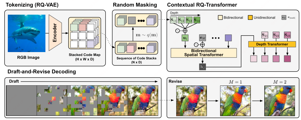
RQVAE tokenization

The first stage of the Contextual RQ-Transformer employs the RQ-VAE—a powerful tokenizer capable of condensing high-dimensional data into a discrete set of latent tokens.

Bidirectional context integration

Once the data is tokenized, the Contextual RQ-Transformer performs two key operations to model the relationships within the tokenized sequence:

1. Bidirectional Spatial Attention: Utilizing bidirectional attention mechanisms, the model predicts the masked positions in the sequence, given a masked scheduling function. This approach allows the model to consider both past and future context, leading to a more accurate and coherent understanding of the data.

2. Autoregressive Depth: The model employs autoregressive transformers to process the sequence depth-wise. This structure is akin to modifying the lower layers of a RQ-Transformer⁸ from a causal (unidirectional) to a bidirectional model. By doing so, the contextual RQ-Transformer captures the sequential dependencies with greater precision.

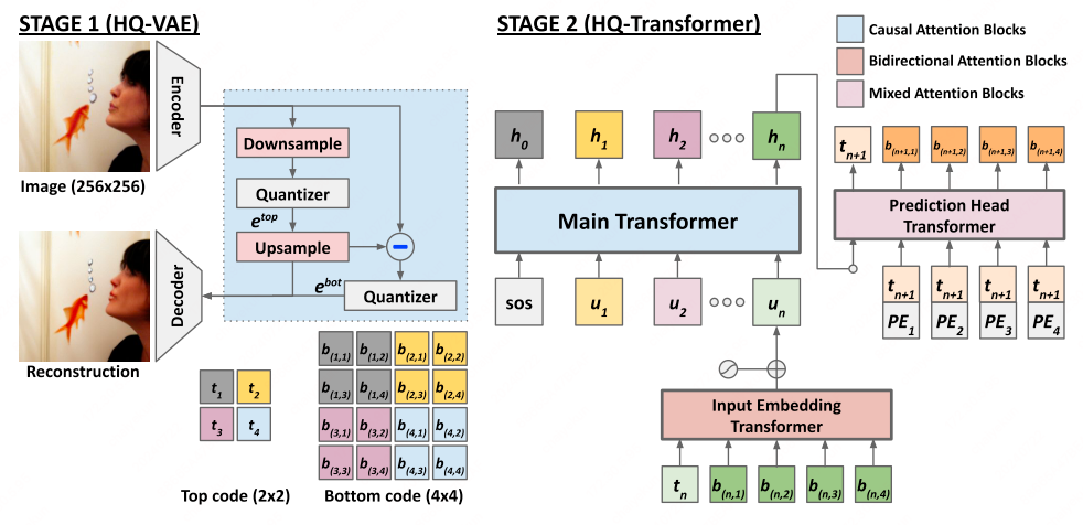
HQ-VAE (NeurIPS’22)

HQ-VAE¹⁰ adopts a hierarchical VQ scheme to encode input data using two levels of discrete codes: top $\mathbf{t}$ and bottom $\mathbf{b}$. It transforms the feature map $\mathbf{z} \in \mathbb{R}^{rl \times rl \times d}$ into two code maps $(\mathbf{t}, \mathbf{b})$, where $\mathbf{t} \in \mathcal{Z}^{l\times l}$ and $\mathbf{b} \in \mathcal{Z}^{rl\times rl}$ with an integer scaling factor $r \in \{1,2,\cdots \}$.

It first captures the high-level information of a feature map by quantizing its downsampled version using the top codes:

where $\mathcal{C}^{\mathrm{top}}$ is the codebook of top codes. Then given the top code map $\mathbf{t}$, the bottom codes are derived at:

where $\mathcal{C}^{\mathrm{bot}}$ is the codebook of bottom codes.

LFQ (MagViT-V2; ICLR’24)

MagViT-V2¹¹ proposes lookup-free quantization (LFQ), which assumes independent codebook dimensions and binary latents. Specifically, the latent space of LFQ is decomposed as the Cartesian product of single-dimensional variables: \(\mathbb{C}=\times_{i=1}^{\log_{2} K}C_{i}\). Given a feature vector \(\mathbf{z} \in \mathbb{R}^{\log_2 K}\), each dimension of the quantized representation $q(\mathbf{z})$ is obtained from:

where \(C_{i,j}\) is the $j$-th value in \(C_i\). With \(C_i = \\{-1,1\\}\), the $\arg\min$ can be computed by the sign function as:

With LFQ, the token index for $q(\mathbf{z})$ is given by:

where \(\vert C_0\vert=1\) sets the virtual basis.

It adds an entropy penalty during training to encourage codebook utilization:

1
2
3
4
5
6
7
8
9
10
11
12
13
14
15
16
17
18
19
20
21
22
23
24
25
26
27
28
29
30
31
32
33
34
35
36
37
38
39
40
41
42
43
44
45
46
47
48
49
50
51
52
53
54
55
56
57
58
59
60
61
62
63
64
65
66
67
68
69
70
71
72
73
74
75
76
77
78
79
80
81
82
83
84
85
86
87
88
89
90
91
92
93
94
95
96
97
98
99
100
101
102
103
104
105
106
107
108
109
110
111
112
113
114
115
116
117
118
119
120
121
122
123
124
125
126
127
128
129
130
131
132
133
134
135
136
137
138
139
140
141
142
143
144
145
146
147
148
149
150
151
152
153
154
155
156
157
158
159
160
161
162
163
164
165
166
167
168
169
170
171
172
173
174
175
176
177
178
179
180
181
182
183
184
185
186
187
188
189
190
191
192
193
194
195
196
197
198
199
200
201
202
203
204
205
206
207
208
209
210
211
212
213
214
215
216
217
218
219
220
221
222
223
224
225
226
227
228
229
230
231
232
233
234
235
236
237
238
239
240
241
242
243
244
245
246
247
248
249
250
251
252
253
254
255
256
257
258
259
260
261
262
263
264
265
266
267
268
269
270
271
272
273
274
275
276
277
278
279
280
281
282
283
284
285
286
287
288
289
290
291
292
293
294
295
296
297
298
299
300
301
302
303
 
"""
Lookup Free Quantization
Proposed in https://arxiv.org/abs/2310.05737

In the simplest setup, each dimension is quantized into {-1, 1}.
An entropy penalty is used to encourage utilization.
"""

from math import log2, ceil
from collections import namedtuple

import torch
from torch import nn, einsum
import torch.nn.functional as F
from torch.nn import Module
from torch.cuda.amp import autocast

from einops import rearrange, reduce, pack, unpack

# constants

Return = namedtuple('Return', ['quantized', 'indices', 'entropy_aux_loss'])

LossBreakdown = namedtuple('LossBreakdown', ['per_sample_entropy', 'batch_entropy', 'commitment'])

# helper functions

def exists(v):
    return v is not None

def default(*args):
    for arg in args:
        if exists(arg):
            return arg() if callable(arg) else arg
    return None

def pack_one(t, pattern):
    return pack([t], pattern)

def unpack_one(t, ps, pattern):
    return unpack(t, ps, pattern)[0]

# entropy

def log(t, eps = 1e-5):
    return t.clamp(min = eps).log()

def entropy(prob):
    return (-prob * log(prob)).sum(dim=-1)

# class

class LFQ(Module):
    def __init__(
        self,
        *,
        dim = None,
        codebook_size = None,
        entropy_loss_weight = 0.1,
        commitment_loss_weight = 0.25,
        diversity_gamma = 1.,
        straight_through_activation = nn.Identity(),
        num_codebooks = 1,
        keep_num_codebooks_dim = None,
        codebook_scale = 1.,            # for residual LFQ, codebook scaled down by 2x at each layer
        frac_per_sample_entropy = 1.    # make less than 1. to only use a random fraction of the probs for per sample entropy
    ):
        super().__init__()

        # some assert validations

        assert exists(dim) or exists(codebook_size), 'either dim or codebook_size must be specified for LFQ'
        assert not exists(codebook_size) or log2(codebook_size).is_integer(), f'your codebook size must be a power of 2 for lookup free quantization (suggested {2 ** ceil(log2(codebook_size))})'

        codebook_size = default(codebook_size, lambda: 2 ** dim)
        codebook_dim = int(log2(codebook_size))

        codebook_dims = codebook_dim * num_codebooks
        dim = default(dim, codebook_dims)

        has_projections = dim != codebook_dims
        self.project_in = nn.Linear(dim, codebook_dims) if has_projections else nn.Identity()
        self.project_out = nn.Linear(codebook_dims, dim) if has_projections else nn.Identity()
        self.has_projections = has_projections

        self.dim = dim
        self.codebook_dim = codebook_dim
        self.num_codebooks = num_codebooks

        keep_num_codebooks_dim = default(keep_num_codebooks_dim, num_codebooks > 1)
        assert not (num_codebooks > 1 and not keep_num_codebooks_dim)
        self.keep_num_codebooks_dim = keep_num_codebooks_dim

        # straight through activation

        self.activation = straight_through_activation

        # entropy aux loss related weights

        assert 0 < frac_per_sample_entropy <= 1.
        self.frac_per_sample_entropy = frac_per_sample_entropy

        self.diversity_gamma = diversity_gamma
        self.entropy_loss_weight = entropy_loss_weight

        # codebook scale

        self.codebook_scale = codebook_scale

        # commitment loss

        self.commitment_loss_weight = commitment_loss_weight

        # for no auxiliary loss, during inference

        self.register_buffer('mask', 2 ** torch.arange(codebook_dim - 1, -1, -1))
        self.register_buffer('zero', torch.tensor(0.), persistent = False)

        # codes

        all_codes = torch.arange(codebook_size)
        bits = ((all_codes[..., None].int() & self.mask) != 0).float()
        codebook = self.bits_to_codes(bits)

        self.register_buffer('codebook', codebook, persistent = False)

    def bits_to_codes(self, bits):
        return bits * self.codebook_scale * 2 - self.codebook_scale # [-1 ,1]

    @property
    def dtype(self):
        return self.codebook.dtype

    def indices_to_codes(
        self,
        indices,
        project_out = True
    ):
        is_img_or_video = indices.ndim >= (3 + int(self.keep_num_codebooks_dim))

        if not self.keep_num_codebooks_dim:
            indices = rearrange(indices, '... -> ... 1')

        # indices to codes, which are bits of either -1 or 1

        bits = ((indices[..., None].int() & self.mask) != 0).to(self.dtype)

        codes = self.bits_to_codes(bits)

        codes = rearrange(codes, '... c d -> ... (c d)')

        # whether to project codes out to original dimensions
        # if the input feature dimensions were not log2(codebook size)

        if project_out:
            codes = self.project_out(codes)

        # rearrange codes back to original shape

        if is_img_or_video:
            codes = rearrange(codes, 'b ... d -> b d ...')

        return codes

    @autocast(enabled = False)
    def forward(
        self,
        x,
        inv_temperature = 100.,
        return_loss_breakdown = False,
        mask = None,
    ):
        """
        einstein notation
        b - batch
        n - sequence (or flattened spatial dimensions)
        d - feature dimension, which is also log2(codebook size)
        c - number of codebook dim
        """

        x = x.float()

        is_img_or_video = x.ndim >= 4

        # standardize image or video into (batch, seq, dimension)

        if is_img_or_video:
            x = rearrange(x, 'b d ... -> b ... d')
            x, ps = pack_one(x, 'b * d')

        assert x.shape[-1] == self.dim, f'expected dimension of {self.dim} but received {x.shape[-1]}'

        x = self.project_in(x)

        # split out number of codebooks

        x = rearrange(x, 'b n (c d) -> b n c d', c = self.num_codebooks)

        # quantize by eq 3.

        original_input = x

        codebook_value = torch.ones_like(x) * self.codebook_scale
        quantized = torch.where(x > 0, codebook_value, -codebook_value)

        # use straight-through gradients (optionally with custom activation fn) if training

        if self.training:
            x = self.activation(x)
            x = x + (quantized - x).detach()
        else:
            x = quantized

        # calculate indices

        indices = reduce((x > 0).int() * self.mask.int(), 'b n c d -> b n c', 'sum')

        # entropy aux loss

        if self.training:
            # the same as euclidean distance up to a constant
            distance = -2 * einsum('... i d, j d -> ... i j', original_input, self.codebook)

            prob = (-distance * inv_temperature).softmax(dim = -1)

            # account for mask

            if exists(mask):
                prob = prob[mask]
            else:
                prob = rearrange(prob, 'b n ... -> (b n) ...')

            # whether to only use a fraction of probs, for reducing memory

            if self.frac_per_sample_entropy < 1.:
                num_tokens = prob.shape[0]
                num_sampled_tokens = int(num_tokens * self.frac_per_sample_entropy)
                rand_mask = torch.randn(num_tokens).argsort(dim = -1) < num_sampled_tokens
                per_sample_probs = prob[rand_mask]
            else:
                per_sample_probs = prob

            # calculate per sample entropy

            per_sample_entropy = entropy(per_sample_probs).mean()

            # distribution over all available tokens in the batch

            avg_prob = reduce(per_sample_probs, '... c d -> c d', 'mean')
            codebook_entropy = entropy(avg_prob).mean()

            # 1. entropy will be nudged to be low for each code, to encourage the network to output confident predictions
            # 2. codebook entropy will be nudged to be high, to encourage all codes to be uniformly used within the batch

            entropy_aux_loss = per_sample_entropy - self.diversity_gamma * codebook_entropy
        else:
            # if not training, just return dummy 0
            entropy_aux_loss = per_sample_entropy = codebook_entropy = self.zero

        # commit loss

        if self.training:
            commit_loss = F.mse_loss(original_input, quantized.detach(), reduction = 'none')

            if exists(mask):
                commit_loss = commit_loss[mask]

            commit_loss = commit_loss.mean()
        else:
            commit_loss = self.zero

        # merge back codebook dim

        x = rearrange(x, 'b n c d -> b n (c d)')

        # project out to feature dimension if needed

        x = self.project_out(x)

        # reconstitute image or video dimensions

        if is_img_or_video:
            x = unpack_one(x, ps, 'b * d')
            x = rearrange(x, 'b ... d -> b d ...')

            indices = unpack_one(indices, ps, 'b * c')

        # whether to remove single codebook dim

        if not self.keep_num_codebooks_dim:
            indices = rearrange(indices, '... 1 -> ...')

        # complete aux loss

        aux_loss = entropy_aux_loss * self.entropy_loss_weight + commit_loss * self.commitment_loss_weight

        ret = Return(x, indices, aux_loss)

        if not return_loss_breakdown:
            return ret

        return ret, LossBreakdown(per_sample_entropy, codebook_entropy, commit_loss)

 

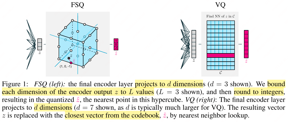
FSQ

Finite Scalar Quantization (FSQ)¹² is a technique that applies a bounding function $f$ to a $d$-dimensional representation $z \in \mathbb{R}^d$, subsequently rounding the result to an integer. The choice of $f$ is critical, as it determines the quantization scheme. Specifically, $f$ is selected such that the output $\hat{z} = \text{round}(f(z))$ can take one of $L$ unique values. An illustrative example of $f$ is given by:

This approach effectively maps $z$ to a quantized representation $\hat{z}$ that belongs to a codebook $\mathcal{C}$, where $\mathcal{C}$ is constructed as the product of per-channel codebook sets. Consequently, the number of distinct codebook entries is given by:

For each vector $\hat{z} \in \mathcal{C}$, there exists a bijective mapping to an integer in the range ${1, \cdots, L^d}$, simplifying the encoding and decoding processes.

Generalized FSQ:

The concept can be further generalized to handle heterogeneous channels, where the $i$-th channel is mapped to \(L_i\) unique values. This generalization yields a more flexible codebook with a total number of entries as follows:

Gradient Propagation via Straight-Through Estimator (STE):

To enable gradient propagation through the discrete round operation, we employ the Straight-Through Estimator (STE) method. This involves replacing the gradients with a simple identity term that ignores the rounding operation during backpropagation. Specifically, the STE-based rounding function is implemented as:

Here, sg represents the stop gradient operation, which blocks gradients from flowing through the second term, effectively treating it as a constant during backpropagation. This allows gradients to “pass through” the rounding operation, enabling training of neural networks utilizing FSQ.

1
2
3
4
 
def round_ste(z: Tensor) -> Tensor:
    """Round with straight through gradients."""
    zhat = z.round()
    return z + (zhat - z).detach()
 

1
2
3
4
5
6
7
8
9
10
11
12
13
14
15
16
17
18
19
20
21
22
23
24
25
26
27
28
29
30
31
32
33
34
35
36
37
38
39
40
41
42
43
44
45
46
47
48
49
50
51
52
53
54
55
56
57
58
59
60
61
62
63
64
65
66
67
68
69
70
71
72
73
74
75
76
77
78
79
80
81
82
83
84
85
86
87
88
89
90
91
92
93
94
95
96
97
98
99
100
101
102
103
104
105
106
107
108
109
110
111
112
113
114
115
116
117
118
119
120
121
122
123
124
125
126
127
128
129
130
131
132
133
134
135
136
137
138
139
140
141
142
143
144
145
146
147
148
149
150
151
152
153
154
155
156
157
158
159
160
161
162
163
164
165
166
167
168
169
170
171
172
173
174
175
176
177
178
179
180
181
182
183
184
185
186
187
188
189
190
191
192
193
194
195
 
"""
Finite Scalar Quantization: VQ-VAE Made Simple - https://arxiv.org/abs/2309.15505
Code adapted from Jax version in Appendix A.1
"""

from typing import List, Tuple, Optional

import torch
import torch.nn as nn
from torch.nn import Module
from torch import Tensor, int32
from torch.cuda.amp import autocast

from einops import rearrange, pack, unpack

# helper functions

def exists(v):
    return v is not None

def default(*args):
    for arg in args:
        if exists(arg):
            return arg
    return None

def pack_one(t, pattern):
    return pack([t], pattern)

def unpack_one(t, ps, pattern):
    return unpack(t, ps, pattern)[0]

# tensor helpers

def round_ste(z: Tensor) -> Tensor:
    """Round with straight through gradients."""
    zhat = z.round()
    return z + (zhat - z).detach()

# main class

class FSQ(Module):
    def __init__(
        self,
        levels: List[int],
        dim: Optional[int] = None,
        num_codebooks = 1,
        keep_num_codebooks_dim: Optional[bool] = None,
        scale: Optional[float] = None,
        allowed_dtypes: Tuple[torch.dtype, ...] = (torch.float32, torch.float64)
    ):
        super().__init__()
        _levels = torch.tensor(levels, dtype=int32)
        self.register_buffer("_levels", _levels, persistent = False)

        _basis = torch.cumprod(torch.tensor([1] + levels[:-1]), dim=0, dtype=int32)
        self.register_buffer("_basis", _basis, persistent = False)

        self.scale = scale

        codebook_dim = len(levels)
        self.codebook_dim = codebook_dim

        effective_codebook_dim = codebook_dim * num_codebooks
        self.num_codebooks = num_codebooks
        self.effective_codebook_dim = effective_codebook_dim

        keep_num_codebooks_dim = default(keep_num_codebooks_dim, num_codebooks > 1)
        assert not (num_codebooks > 1 and not keep_num_codebooks_dim)
        self.keep_num_codebooks_dim = keep_num_codebooks_dim

        self.dim = default(dim, len(_levels) * num_codebooks)

        has_projections = self.dim != effective_codebook_dim
        self.project_in = nn.Linear(self.dim, effective_codebook_dim) if has_projections else nn.Identity()
        self.project_out = nn.Linear(effective_codebook_dim, self.dim) if has_projections else nn.Identity()
        self.has_projections = has_projections

        self.codebook_size = self._levels.prod().item()

        implicit_codebook = self.indices_to_codes(torch.arange(self.codebook_size), project_out = False)
        self.register_buffer("implicit_codebook", implicit_codebook, persistent = False)

        self.allowed_dtypes = allowed_dtypes

    def bound(self, z: Tensor, eps: float = 1e-3) -> Tensor:
        """Bound `z`, an array of shape (..., d)."""
        half_l = (self._levels - 1) * (1 + eps) / 2
        offset = torch.where(self._levels % 2 == 0, 0.5, 0.0)
        shift = (offset / half_l).atanh()
        return (z + shift).tanh() * half_l - offset

    def quantize(self, z: Tensor) -> Tensor:
        """Quantizes z, returns quantized zhat, same shape as z."""
        quantized = round_ste(self.bound(z))
        half_width = self._levels // 2 # Renormalize to [-1, 1].
        return quantized / half_width

    def _scale_and_shift(self, zhat_normalized: Tensor) -> Tensor:
        half_width = self._levels // 2
        return (zhat_normalized * half_width) + half_width

    def _scale_and_shift_inverse(self, zhat: Tensor) -> Tensor:
        half_width = self._levels // 2
        return (zhat - half_width) / half_width

    def codes_to_indices(self, zhat: Tensor) -> Tensor:
        """Converts a `code` to an index in the codebook."""
        assert zhat.shape[-1] == self.codebook_dim
        zhat = self._scale_and_shift(zhat)
        return (zhat * self._basis).sum(dim=-1).to(int32)

    def indices_to_codes(
        self,
        indices: Tensor,
        project_out = True
    ) -> Tensor:
        """Inverse of `codes_to_indices`."""

        is_img_or_video = indices.ndim >= (3 + int(self.keep_num_codebooks_dim))

        indices = rearrange(indices, '... -> ... 1')
        codes_non_centered = (indices // self._basis) % self._levels
        codes = self._scale_and_shift_inverse(codes_non_centered)

        if self.keep_num_codebooks_dim:
            codes = rearrange(codes, '... c d -> ... (c d)')

        if project_out:
            codes = self.project_out(codes)

        if is_img_or_video:
            codes = rearrange(codes, 'b ... d -> b d ...')

        return codes

    @autocast(enabled = False)
    def forward(self, z: Tensor) -> Tensor:
        """
        einstein notation
        b - batch
        n - sequence (or flattened spatial dimensions)
        d - feature dimension
        c - number of codebook dim
        """

        orig_dtype = z.dtype
        is_img_or_video = z.ndim >= 4

        # standardize image or video into (batch, seq, dimension)

        if is_img_or_video:
            z = rearrange(z, 'b d ... -> b ... d')
            z, ps = pack_one(z, 'b * d')

        assert z.shape[-1] == self.dim, f'expected dimension of {self.dim} but found dimension of {z.shape[-1]}'

        z = self.project_in(z)

        z = rearrange(z, 'b n (c d) -> b n c d', c = self.num_codebooks)

        # make sure allowed dtype before quantizing

        if z.dtype not in self.allowed_dtypes:
            z = z.float()

        codes = self.quantize(z)
        indices = self.codes_to_indices(codes)

        codes = rearrange(codes, 'b n c d -> b n (c d)')

        # cast codes back to original dtype

        if codes.dtype != orig_dtype:
            codes = codes.type(orig_dtype)

        # project out

        out = self.project_out(codes)

        # reconstitute image or video dimensions

        if is_img_or_video:
            out = unpack_one(out, ps, 'b * d')
            out = rearrange(out, 'b ... d -> b d ...')

            indices = unpack_one(indices, ps, 'b * c')

        if not self.keep_num_codebooks_dim:
            indices = rearrange(indices, '... 1 -> ...')

        # return quantized output and indices

        return out, indices

 

Related work: Binary Spherical Quantization (BSQ)¹³.

Prior Learning

In the second stage, existing methods typically apply causal or bidirectional language models for prior learning over the discrete latent codes.

Causal Transformer Modeling

This approach trains an autoregressive language model over the quantized tokens, as in VQGAN⁴, ViT-VQGAN⁷, DALL-E⁶, and iGPT⁵.

Bidirectional Transformer Modeling

An alternative approach uses bidirectional modeling for image prior learning, as in MaskGIT¹⁴, MagViT-V2¹¹, and Muse¹⁵.

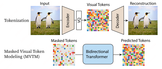
MaskGIT (CVPR’22)

MaskGIT¹⁴ consists of two stages:

1. VQ tokenizer training as in VQGAN;
2. Masked Visual Token Modeling (MVTM) on a bidirectional transformer.

Masked Visual Token Modeling (MVTM)

MaskGIT uses a mask scheduling function to strategically mask input latent tokens in a bidirectional transformer. The masked tokens are predicted via cross-entropy loss against the ground truth, closely resembling masked language modeling.

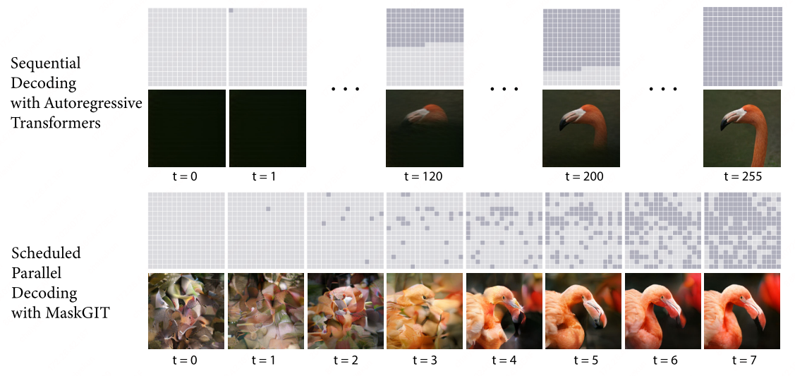
Iterative Decoding

Autoregressive decoding is inherently sequential and slow. MaskGIT overcomes this with bidirectional parallel decoding:

Decoding Process:

(1) Predict. At each iteration $t$, MaskGIT utilizes the current masked tokens \(Y_M^{(t)}\) to predict probabilities $p^{(t)} \in \mathbb{R}^{N \times K}$ for all masked locations in parallel. This step leverages the capabilities of bidirectional transformers to simultaneously assess potential replacements for each masked token.

(2) Sample. For each masked location $i$, MaskGIT samples tokens \(y_i^{(t)}\) based on the predicted probabilities \(p_i^{(t)} \in \mathbb{R}^{K}\) over all possible tokens in the codebook. The sampled token’s prediction score serves as a “confidence” score, indicating the model’s certainty in its prediction. For unmasked positions in \(Y_M^{(t)}\), the confidence score is set to 1.0, representing absolute certainty.

(3) Mask Schedule. The number of tokens to mask at iteration $t$ is determined using the mask scheduling function $\gamma$:

Here, $N$ is the input length, $T$ is the total number of iterations, and $n$ is the number of tokens to be masked. As $t$ progresses, $\gamma$ ensures a decreasing mask ratio, allowing the model to gradually generate more tokens until all are uncovered within $T$ steps.

(4) Mask. To obtain \(Y_M^{(t+1)}\) for iteration $t+1$, MaskGIT masks $n$ tokens in \(Y_M^{(t)}\) based on their confidence scores. The mask $M^{(t+1)}$ is calculated as follows:

where \(c_i\) is the confidence score for the $i$-th token, and \(\text{sorted}_j(c_j)[n]\) represents the $n$-th smallest confidence score among all tokens.

Synthesis in $T$ steps: MaskGIT generates an image in $T$ iterations. At each step, probabilities are predicted for all masked tokens in parallel, but only the most confident predictions are kept. The rest are re-masked and re-predicted in the next iteration. The progressively decreasing mask ratio ensures all tokens are uncovered within $T$ steps.

References