Diffusion Models: A Mathematical Guide from Scratch

Diffusion models have reshaped generative AI—yet beneath the impressive samples lies a surprisingly coherent mathematical framework. At its core, the idea is disarmingly simple: systematically destroy structure through a fixed noise process, then learn to reverse it step by step. What makes this work is a deep connection between three seemingly distinct perspectives: variational inference (ELBO optimization), score matching (learning \(\nabla_\mathbf{x} \log p(\mathbf{x})\)), and stochastic differential equations.

This post is a self-contained mathematical walkthrough, written to be the reference I wished I had when first deriving these results. We start from the Gaussian forward process, carefully derive the reverse posterior and its closed-form mean, then trace how the ELBO decomposes into tractable KL terms. From there, we cover the three prediction parameterizations (\(\mathbf{x}_0\), $\pmb{\epsilon}$, and velocity $\mathbf{v}$), classifier and classifier-free guidance for conditional generation, and finally extend the entire framework to categorical (discrete) state spaces via D3PM transition matrices.

Every equation is derived rather than stated—if you want to understand why the simplified loss drops the weighting term, or how classifier-free guidance implicitly sharpens the conditional score, the derivations are here.

Gaussian Diffusion (Continuous)

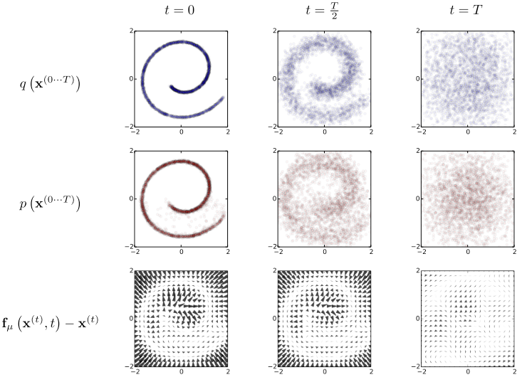
Diffusion models¹² are latent variable models inspired by non-equilibrium statistical physics (thermodynamics). They gradually destroy structure in the data distribution through an iterative forward diffusion process, then learn to reverse it step by step via iterative denoising.

Diffusion models can be treated as a Markovian Hierarchical Variational Autoencoder with three restrictions:³

1. The latent dimension is the same as the original data.
2. The encoder is not learned, instead uses a (pre-defined) linear Gaussian model.
3. The latent in final timestep $T$ is an isotropic Gaussian.

Forward (Diffusion) process

Given a data point sampled from the data distribution \(\mathbf{x}_0 \sim q(\mathbf{x})\), the forward diffusion process applies a fixed linear Gaussian model at each timestep $t$ out of $T$ steps:

\[\begin{align} q(\mathbf{x}_t \vert \mathbf{x}_{t-1}) = \mathcal{N} (\mathbf{x}_t; \sqrt{1-\beta_t} \mathbf{x}_{t-1}, \beta_t \mathbf{I}) \end{align}\]

where the forward transitions produce a series of progressively noisier samples \(\mathbf{x}_1, \cdots, \mathbf{x}_T\). Each sample has exactly the same dimensionality as the original data point \(\mathbf{x}_0\).

Under the Markovian assumption, Gaussian noise is incrementally added to the sample from the previous timestep according to a variance schedule \(\{\beta_t \in (0, 1) \}_{t=1}^T\). As $T \to \infty$, \(\mathbf{x}_T\) approaches an isotropic Gaussian distribution.

Let \(\alpha_t = 1 - \beta_t\), the linear Gaussian model in the forward process is rewritten as:

\[\begin{align} q(\mathbf{x}_t \vert \mathbf{x}_{t-1}) = \mathcal{N} (\mathbf{x}_t; \sqrt{\alpha_t} \mathbf{x}_{t-1}, (1-\alpha_t) \mathbf{I}) \end{align}\]

Under the reparameterization trick, samples \(\mathbf{x}_t \sim q (\mathbf{x}_t \vert \mathbf{x}_{t-1})\) can be rewritten as:

\[\begin{align} \mathbf{x}_t = \sqrt{\alpha_t} \mathbf{x}_{t-1} + \sqrt{1-\alpha_t} \pmb{\epsilon} \,\,\,\, \text{with } \,\,\,\, \pmb{\epsilon}\sim \mathcal{N} (\pmb{\epsilon}; \mathbf{0},\mathbf{I}) \end{align}\]

In similar vein, samples \(\mathbf{x}_{t-1}\) can be rewritten as:

\[\begin{align} \mathbf{x}_{t-1} = \sqrt{\alpha_{t-1}} \mathbf{x}_{t-2} + \sqrt{1-\alpha_{t-1}} \pmb{\epsilon} \,\,\,\, \text{with } \,\,\,\, \pmb{\epsilon}\sim \mathcal{N} (\pmb{\epsilon}; \mathbf{0},\mathbf{I}) \end{align}\]

Let

\[\bar{\alpha}_t = \prod_{i=1}^t \alpha_i.\]

Typically, the noise magnitude increases with the timestep, i.e.,

\[\beta_1 < \beta_2 < \cdots < \beta_T \quad \text{and thus} \quad \bar{\alpha}_1 > \bar{\alpha}_2 > \cdots > \bar{\alpha}_T.\]

Suppose we have $2T$ random noise variables

\[\{ \pmb{\epsilon}_t, \bar{\pmb{\epsilon}}_t \}_{t=1}^T \overset{\text{i.i.d}}{\sim} \mathcal{N} (\pmb{\epsilon}; \mathbf{0},\mathbf{I}).\]

For an arbitrary sample \(\mathbf{x}_t \sim q(\mathbf{x}_t \vert \mathbf{x}_0)\), we have:

\[\begin{align} \mathbf{x}_t &{}= \sqrt{\alpha_t} \mathbf{x}_{t-1} + \sqrt{1-\alpha_t} \pmb{\epsilon}_{t-1} \\ &{}= \sqrt{\alpha_t} (\sqrt{\alpha_{t-1}} \mathbf{x}_{t-2} + \sqrt{1-\alpha_{t-1}} \pmb{\epsilon}_{t-2}) + \sqrt{1-\alpha_{t}} \pmb{\epsilon}_{t-1} \nonumber \\ &{}= \sqrt{\alpha_t \alpha_{t-1}} \mathbf{x}_{t-2} + \sqrt{\alpha_t- \alpha_t \alpha_{t-1}} \pmb{\epsilon}_{t-2} + \sqrt{1-\alpha_{t}} \pmb{\epsilon}_{t-1} \nonumber \\ &{}= \sqrt{\alpha_t \alpha_{t-1}} \mathbf{x}_{t-2} + \sqrt{\sqrt{\alpha_t- \alpha_t \alpha_{t-1}}^2 + \sqrt{1-\alpha_{t}}^2 } \bar{\pmb{\epsilon}}_{t-2}) \nonumber \\ &{}= \sqrt{\alpha_t \alpha_{t-1}} \mathbf{x}_{t-2} + \sqrt{1 - \alpha_t \alpha_{t-1}} \bar{\pmb{\epsilon}}_{t-2})\\ &{}= \cdots \nonumber \\ &{}= \sqrt{\prod_{i=1}^t \alpha_i \mathbf{x}_0} + \sqrt{1 - \prod_{i=1}^t \alpha_i \pmb{\epsilon}_0} \\ &{}= \color{blue}{\sqrt{\bar{\alpha}_t} \mathbf{x}_0 + \sqrt{1-\bar{\alpha}_t} \bar{\pmb{\epsilon}}_0} \label{forward_add_noise} \\ &{} \sim \mathcal{N} (\mathbf{x}_t; \sqrt{\bar{\alpha}_t} \mathbf{x}_0, (1-\bar{\alpha}_t) \mathbf{I}) \label{noise_process} \end{align}\]

Therefore, we obtain the closed-form marginal: \(q(\mathbf{x}_t \vert \mathbf{x}_0) = \mathcal{N} (\mathbf{x}_t; \sqrt{\bar{\alpha}_t} \mathbf{x}_0, (1-\bar{\alpha}_t) \mathbf{I})\).

Reverse process

The reverse diffusion process, with the marginal \(p_\theta(\mathbf{x}_0) := \int p_\theta (\mathbf{x}_{0:T}) \, d \mathbf{x}_{1:T}\), learns to invert the forward process by gradually denoising from timestep $T$ to $1$. It is defined as a Markov chain with learned Gaussian transitions starting at \(p(\mathbf{x}_T) = \mathcal{N}(\mathbf{x}_T; \mathbf{0}, \mathbf{I})\):

\[\begin{align} p_\theta (\mathbf{x}_{0:T}) &{}:= p(\mathbf{x}_T) \prod_{t=1}^T p_\theta (\mathbf{x}_{t-1}\vert \mathbf{x}_t) \\ p_\theta (\mathbf{x}_{t-1}\vert\mathbf{x}_{t}) &{} := \mathcal{N} (\mathbf{x}_{t-1}; \pmb{\mu}_\theta (\mathbf{x}_{t},t), \pmb{\Sigma}_\theta (\mathbf{x}_{t}, t)) \end{align}\]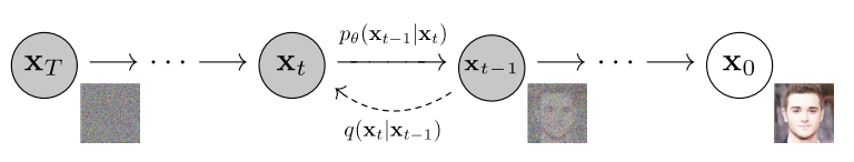

We can derive the Gaussian form of both \(q(\mathbf{x}_t \vert \mathbf{x}_0)\) and \(q(\mathbf{x}_{t-1} \vert \mathbf{x}_0)\). Applying Bayes’ rule, we obtain:

\[\begin{align} q(\mathbf{x}_{t-1} \vert \mathbf{x}_t, \mathbf{x}_0) &{}= \frac{q(\mathbf{x}_t \vert \mathbf{x}_{t-1}, \mathbf{x}_0) \cdot q(\mathbf{x}_{t-1} \vert \mathbf{x}_0)}{q(\mathbf{x}_t \vert \mathbf{x}_0)} \\ &{}= \frac{\mathcal{N} (\mathbf{x}_t; \sqrt{\alpha_t} \mathbf{x}_0, (1-\alpha_t) \mathbf{I}) \cdot \mathcal{N} (\mathbf{x}_{t-1}; \sqrt{\bar{\alpha}_{t-1}} \mathbf{x}_0, (1-\bar{\alpha}_{t-1}) \mathbf{I})}{\mathcal{N} (\mathbf{x}_t; \sqrt{\bar{\alpha}_t} \mathbf{x}_0, (1-\bar{\alpha}_t) \mathbf{I})} \\ &{}\propto \exp \big\{ -\frac{1}{2} ( \frac{(\mathbf{x}_t - \sqrt{\alpha} \mathbf{x}_{t-1})^2}{1-\alpha_t} + \frac{(\mathbf{x}_{t-1} - \sqrt{\bar{\alpha}_{t-1}}\mathbf{x}_0)^2}{1-\bar{\alpha}_{t-1}} + \frac{(\mathbf{x}_t - \sqrt{\bar{\alpha}_t} \mathbf{x}_0)^2}{1-\bar{\alpha}_t} ) \big\} \\ &{}= \exp \big\{ -\frac{1}{2} (\frac{-2\sqrt{\alpha_t} \mathbf{x}_t \mathbf{x}_{t-1} + \alpha_t \mathbf{x}_{t-1}^2 }{ 1 - \alpha_t} ) + \frac{\mathbf{x}_{t-1}^2 - 2 \sqrt{\bar{\alpha}_{t-1}}\mathbf{x}_{t-1}\mathbf{x}_0}{1-\bar{\alpha}_{t-1}} + C(\mathbf{x}_t, \mathbf{x}_0) \big\} \\ &{}\propto \exp\Big\{ -\frac{1}{2} \big( (\frac{\alpha_t}{1-\alpha_t} + \frac{1}{1 - \bar{\alpha}_{t-1}}) \mathbf{x}_{t-1}^2 - 2(\frac{\sqrt{\alpha_t}}{1-\alpha_t} \mathbf{x}_t + \frac{\sqrt{\bar{\alpha}_{t-1}}}{1 - \bar{\alpha}_{t-1}} \mathbf{x}_0) \mathbf{x}_{t-1} \big) \Big\} \\ &{}= \exp\Big\{ -\frac{1}{2} (\frac{1}{\frac{(1-\alpha_t)(1-\bar{\alpha}_{t-1})}{1-\bar{\alpha}_t}}) \Big[ \mathbf{x}_{t-1}^2 - 2\frac{\sqrt{\alpha_t} (1-\bar{\alpha}_{t-1})\mathbf{x}_t + \sqrt{\bar{\alpha}_{t-1}}(1-\alpha_t)\mathbf{x}_0 }{1-\bar{\alpha}_t} \mathbf{x}_{t-1}\Big] \Big\} \\ &{}\propto \mathcal{N}\Big(\mathbf{x}_{t-1}; \underbrace{\frac{\sqrt{\alpha_t} (1-\bar{\alpha}_{t-1})\mathbf{x}_t + \sqrt{\bar{\alpha}_{t-1}}(1-\alpha_t)\mathbf{x}_0 }{1-\bar{\alpha}_t}}_{\color{blue}{\pmb{\mu}(\mathbf{x}_t, \mathbf{x}_0)}}, \underbrace{\frac{(1-\alpha_t)(1-\bar{\alpha}_{t-1})}{1-\bar{\alpha}_t}}_{\color{green}{\pmb{\Sigma}_q(t)}} \Big) \label{mu} \end{align}\]

At each timestep, \(\mathbf{x}_{t-1} \sim q(\mathbf{x}_{t-1} \vert \mathbf{x}_t, \mathbf{x}_0)\) follows a Gaussian distribution. The mean \(\pmb{\mu}(\mathbf{x}_t, \mathbf{x}_0)\) is a function of \(\mathbf{x}_t\) and \(\mathbf{x}_0\), while \(\pmb{\Sigma}_q(t)\) depends only on the $\alpha$ schedule (either fixed as a hyperparameter or learned). The variance takes the form \(\pmb{\Sigma}_q (t) = \sigma^2_q (t) \mathbf{I}\), where \(\sigma^2_q(t)=\frac{(1-\alpha_t)(1-\bar{\alpha}_{t-1})}{1-\bar{\alpha}_t}\).

Since \(p_\theta(\mathbf{x}_{t-1} \vert \mathbf{x}_t)\) does not condition on \(\mathbf{x}_0\), we optimize the KL divergence between the two Gaussian distributions, which reduces to matching their means:

\[\begin{align} &{}\mathop{\arg\min}_\theta \; D_\text{KL} \Big( q(\mathbf{x}_{t-1}\vert \mathbf{x}_t, \mathbf{x}_0) \Vert p_\theta (\mathbf{x}_{t-1} \vert \mathbf{x}_t) \Big) \\ = &{}\mathop{\arg\min}_\theta \; D_\text{KL} \Big( \mathcal{N} \big( \mathbf{x}_{t-1}; \pmb{\mu}_q, \pmb{\Sigma}_q(t) \big) \Vert \mathcal{N} \big( \mathbf{x}_{t-1}; \pmb{\mu}_\theta, \pmb{\Sigma}_q(t) \big) \Big) \\ = &{}\mathop{\arg\min}_\theta \; \frac{1}{2} \Big[ \log \frac{\vert\pmb{\Sigma}_q (t)\vert}{\vert \pmb{\Sigma}_q (t)\vert} -d + \text{tr} (\pmb{\Sigma}_q (t)^{-1} \Sigma_q (t)) + (\pmb{\mu}_\theta - \pmb{\mu}_q)^T \pmb{\Sigma}_q (t)^{-1} (\pmb{\mu}_\theta - \pmb{\mu}_q) \Big] \\ = &{}\mathop{\arg\min}_\theta \; \frac{1}{2} \Big[ \log 1 -d + d + (\pmb{\mu}_\theta - \pmb{\mu}_q)^T \pmb{\Sigma}_q (t)^{-1} (\pmb{\mu}_\theta - \pmb{\mu}_q) \Big] \\ = &{}\mathop{\arg\min}_\theta \;\frac{1}{2} \Big[ (\pmb{\mu}_\theta - \pmb{\mu}_q)^T \Sigma_q (t)^{-1} (\pmb{\mu}_\theta - \pmb{\mu}_q) \Big] \\ = &{}\mathop{\arg\min}_\theta \;\frac{1}{2} \Big[ (\pmb{\mu}_\theta - \pmb{\mu}_q)^T (\sigma_q^2 (t)\mathbf{I})^{-1} (\pmb{\mu}_\theta - \pmb{\mu}_q) \Big] \\ = &{}\mathop{\arg\min}_\theta \; \frac{1}{2 \sigma_q^2 (t)} \Vert \pmb{\mu}_\theta - \pmb{\mu}_q \Vert_2^2 \label{kl} \end{align}\]

Given Eq.$\eqref{mu}$, we have:

\[\begin{align} \pmb{\mu}_q (\mathbf{x}_t, \mathbf{x}_0) &{}= \frac{\sqrt{\alpha_t} (1-\bar{\alpha}_{t-1})\mathbf{x}_t + \sqrt{\bar{\alpha}_{t-1}}(1-\alpha_t) \color{green}{\mathbf{x}_0} }{1-\bar{\alpha}_t} \label{mu_q} \\ \pmb{\mu}_\theta (\mathbf{x}_t, t) &{}= \frac{\sqrt{\alpha_t} (1-\bar{\alpha}_{t-1})\mathbf{x}_t + \sqrt{\bar{\alpha}_{t-1}}(1-\alpha_t) \color{blue}{\hat{\mathbf{x}}_\theta (\mathbf{x}_t, t)} }{1-\bar{\alpha}_t} \label{mu_theta} \\ \end{align}\]

Therefore, Eq.$\eqref{kl}$ can be rewritten as:

\[\begin{align} &{}\mathop{\arg\min}_\theta \; D_\text{KL} \Big( q(\mathbf{x}_{t-1}\vert \mathbf{x}_t, \mathbf{x}_0) \Vert p_\theta (\mathbf{x}_{t-1} \vert \mathbf{x}_t) \Big) \\ = &{}\mathop{\arg\min}_\theta \; D_\text{KL} \Big( \mathcal{N} \big( \mathbf{x}_{t-1}; \pmb{\mu}_q, \pmb{\Sigma}_q(t) \big) \Vert \mathcal{N} \big( \mathbf{x}_{t-1}; \pmb{\mu}_\theta, \pmb{\Sigma}_q(t) \big) \Big) \\ = &{}\mathop{\arg\min}_\theta \; \frac{1}{2\sigma_q^2 (t)} \big\Vert \frac{\sqrt{\bar{\alpha}_{t-1}}(1-\alpha_t) \hat{\mathbf{x}}_\theta (\mathbf{x}_t, t) }{1-\bar{\alpha}_t} - \frac{\sqrt{\bar{\alpha}_{t-1}}(1-\alpha_t) \mathbf{x}_0 }{1-\bar{\alpha}_t} \big\Vert_2^2 \\ = &{}\mathop{\arg\min}_\theta \; \frac{1}{2\sigma_q^2 (t)} \big\Vert \frac{\sqrt{\bar{\alpha}_{t-1}}(1-\alpha_t) }{1-\bar{\alpha}_t} (\hat{\mathbf{x}}_\theta (\mathbf{x}_t, t) - \mathbf{x}_0) \big\Vert_2^2 \\ = &{}\mathop{\arg\min}_\theta \; \frac{1}{2\sigma_q^2 (t)} \frac{\bar{\alpha}_{t-1}(1-\alpha_t)^2 }{(1-\bar{\alpha}_t)^2} \big\Vert (\hat{\mathbf{x}}_\theta (\mathbf{x}_t, t) - \mathbf{x}_0) \big\Vert_2^2 \label{loss_mu} \end{align}\]

Intuitive understanding towards the diffusion process¹³.

\[\begin{align} \log p(\mathbf{x}) &{}= \log \int p(\mathbf{x}_{0:T}) d \mathbf{x}_{1:T} \\ &{}= \log \int \frac{ p(\mathbf{x}_{0:T}) q(\mathbf{x}_{1:T} \vert \mathbf{x}_0)}{q(\mathbf{x}_{1:T} \vert \mathbf{x}_0)} d \mathbf{x}_{1:T} \\ &{}= \log \mathbb{E}_{q(\mathbf{x}_{1:T}\vert\mathbf{x}_0) }\Big[ \frac{p(\mathbf{x}_{0:T}) }{q(\mathbf{x}_{1:T}\vert\mathbf{x}_0)} \Big] \\ &{} \geq \mathbb{E}_{q(\mathbf{x}_{1:T}\vert\mathbf{x}_0) }\Big[ \log \frac{p(\mathbf{x}_{0:T}) }{q(\mathbf{x}_{1:T}\vert\mathbf{x}_0)} \Big] \\ &{} =\mathbb{E}_{q(\mathbf{x}_{1:T}\vert\mathbf{x}_0) }\Big[ \log \frac{p(\mathbf{x}_{T}) \prod_{t=1}^T p_\theta(\mathbf{x}_{t-1}\vert\mathbf{x}_t) }{\prod_{t=1}^T q(\mathbf{x}_t \vert\mathbf{x}_{t-1})} \Big] \\ &{} = \mathbb{E}_{q(\mathbf{x}_{1:T}\vert\mathbf{x}_0) }\Big[ \log \frac{p(\mathbf{x}_{T}) p_\theta( \mathbf{x}_0 \vert \mathbf{x}_1) \prod_{t=2}^T p_\theta(\mathbf{x}_{t-1}\vert\mathbf{x}_t) }{q(\mathbf{x}_T \vert\mathbf{x}_{T-1}) \prod_{t=1}^{T-1} q(\mathbf{x}_t \vert\mathbf{x}_{t-1})} \Big] \\ &{} = \mathbb{E}_{q(\mathbf{x}_{1:T}\vert\mathbf{x}_0) }\Big[ \log \frac{p(\mathbf{x}_{T}) p_\theta ( \mathbf{x}_0 \vert \mathbf{x}_1) \prod_{t=1}^{T-1} p_\theta(\mathbf{x}_{t}\vert\mathbf{x}_{t+1}) }{q(\mathbf{x}_T \vert\mathbf{x}_{T-1}) \prod_{t=1}^{T-1} q(\mathbf{x}_t \vert\mathbf{x}_{t-1})} \Big] \\ &{} = \mathbb{E}_{q(\mathbf{x}_{1:T}\vert\mathbf{x}_0) }\Big[ \log p_\theta( \mathbf{x}_0 \vert \mathbf{x}_1) \Big] + \mathbb{E}_{q(\mathbf{x}_{1:T}\vert\mathbf{x}_0) }\Big[ \log \frac{\log p(\mathbf{x}_T)}{q(\mathbf{x}_T \vert\mathbf{x}_{T-1})} \Big] + \nonumber \\ &{} \qquad\qquad\qquad \quad\quad \sum_{t=1}^{T-1} \mathbb{E}_{q(\mathbf{x}_{1:T}\vert\mathbf{x}_0) }\Big[ \log \frac{p_\theta (\mathbf{x}_t \vert \mathbf{x}_{t+1}) }{ q (\mathbf{x}_t \vert \mathbf{x}_{t-1}) } \Big]\\ &{} = \mathbb{E}_{q(\mathbf{x}_{1}\vert\mathbf{x}_0) }\Big[ \log p_\theta( \mathbf{x}_0 \vert \mathbf{x}_1) \Big] + \mathbb{E}_{q(\mathbf{x}_{T-1}, \mathbf{x}_{T}\vert\mathbf{x}_0) }\Big[ \log \frac{\log p(\mathbf{x}_T)}{q(\mathbf{x}_T \vert\mathbf{x}_{T-1})} \Big] + \nonumber \\ &{} \qquad\qquad\qquad \quad\quad \sum_{t=1}^{T-1} \mathbb{E}_{q(\mathbf{x}_{t-1}, \mathbf{x}_{t}, \mathbf{x}_{t+1}\vert\mathbf{x}_0) }\Big[ \log \frac{p_\theta (\mathbf{x}_t \vert \mathbf{x}_{t+1}) }{ q (\mathbf{x}_t \vert \mathbf{x}_{t-1}) } \Big] \\ &{} = \underbrace{\mathbb{E}_{q(\mathbf{x}_{1}\vert\mathbf{x}_0) }\Big[ \log p_\theta( \mathbf{x}_0 \vert \mathbf{x}_1) \Big]}_{\text{reconstruction}} + \underbrace{\mathbb{E}_{q(\mathbf{x}_{T-1} \vert\mathbf{x}_0) } \Big[ D_\text{KL}(q(\mathbf{x}_T \vert\mathbf{x}_{T-1}) \Vert p(\mathbf{x}_T)) \Big]}_{\text{prior matching} \rightarrow 0} + \nonumber \\ &{} \qquad\qquad\qquad \quad\quad \underbrace{\sum_{t=1}^{T-1} \mathbb{E}_{q(\mathbf{x}_{t-1}, \mathbf{x}_{t}, \mathbf{x}_{t+1}\vert\mathbf{x}_0) }\Big[ \log \frac{p_\theta (\mathbf{x}_t \vert \mathbf{x}_{t+1}) }{ q (\mathbf{x}_t \vert \mathbf{x}_{t-1}) } \Big]}_{\text{consistency}} \end{align}\]

1. The reconstruction term corresponds to the first-step optimization.
2. The prior matching term does not contain trainable parameters, requiring no optimization.
3. The consistency term makes the denoising process at timestep $t$ match the corresponding diffusion step from a cleaner input.

The ELBO objective is thus approximated across all noise levels over the expectation of all timesteps.

Training

The ELBO objective can be derived as ⁴

\[\begin{align} \mathcal{L}_\text{VLB} &{}= - \log p_\theta(\mathbf{x}_0) \\ &\leq - \log p_\theta(\mathbf{x}_0) + D_\text{KL}(q(\mathbf{x}_{1:T}\vert\mathbf{x}_0) \| p_\theta(\mathbf{x}_{1:T}\vert\mathbf{x}_0) ) \\ &= -\log p_\theta(\mathbf{x}_0) + \mathbb{E}_{\mathbf{x}_{1:T}\sim q(\mathbf{x}_{1:T} \vert \mathbf{x}_0)} \Big[ \log\frac{q(\mathbf{x}_{1:T}\vert\mathbf{x}_0)}{p_\theta(\mathbf{x}_{0:T}) / p_\theta(\mathbf{x}_0)} \Big] \\ &= -\log p_\theta(\mathbf{x}_0) + \mathbb{E}_q \Big[ \log\frac{q(\mathbf{x}_{1:T}\vert\mathbf{x}_0)}{p_\theta(\mathbf{x}_{0:T})} + \log p_\theta(\mathbf{x}_0) \Big] \\ &= \mathbb{E}_q \Big[ \log \frac{q(\mathbf{x}_{1:T}\vert\mathbf{x}_0)}{p_\theta(\mathbf{x}_{0:T})} \Big] \\ &= \mathbb{E}_q \Big[ \log\frac{\prod_{t=1}^T q(\mathbf{x}_t\vert\mathbf{x}_{t-1})}{ p_\theta(\mathbf{x}_T) \prod_{t=1}^T p_\theta(\mathbf{x}_{t-1} \vert\mathbf{x}_t) } \Big] \\ &= \mathbb{E}_q \Big[ -\log p_\theta(\mathbf{x}_T) + \sum_{t=1}^T \log \frac{q(\mathbf{x}_t\vert\mathbf{x}_{t-1})}{p_\theta(\mathbf{x}_{t-1} \vert\mathbf{x}_t)} \Big] \\ &= \mathbb{E}_q \Big[ -\log p_\theta(\mathbf{x}_T) + \sum_{t=2}^T \log \frac{q(\mathbf{x}_t\vert\mathbf{x}_{t-1})}{p_\theta(\mathbf{x}_{t-1} \vert\mathbf{x}_t)} + \log\frac{q(\mathbf{x}_1 \vert \mathbf{x}_0)}{p_\theta(\mathbf{x}_0 \vert \mathbf{x}_1)} \Big] \\ &= \mathbb{E}_q \Big[ -\log p_\theta(\mathbf{x}_T) + \sum_{t=2}^T \log \Big( \frac{q(\mathbf{x}_{t-1} \vert \mathbf{x}_t, \mathbf{x}_0)}{p_\theta(\mathbf{x}_{t-1} \vert\mathbf{x}_t)}\cdot \frac{q(\mathbf{x}_t \vert \mathbf{x}_0)}{q(\mathbf{x}_{t-1}\vert\mathbf{x}_0)} \Big) + \log \frac{q(\mathbf{x}_1 \vert \mathbf{x}_0)}{p_\theta(\mathbf{x}_0 \vert \mathbf{x}_1)} \Big] \\ &= \mathbb{E}_q \Big[ -\log p_\theta(\mathbf{x}_T) + \sum_{t=2}^T \log \frac{q(\mathbf{x}_{t-1} \vert \mathbf{x}_t, \mathbf{x}_0)}{p_\theta(\mathbf{x}_{t-1} \vert\mathbf{x}_t)} + \sum_{t=2}^T \log \frac{q(\mathbf{x}_t \vert \mathbf{x}_0)}{q(\mathbf{x}_{t-1} \vert \mathbf{x}_0)} + \log\frac{q(\mathbf{x}_1 \vert \mathbf{x}_0)}{p_\theta(\mathbf{x}_0 \vert \mathbf{x}_1)} \Big] \\ &= \mathbb{E}_q \Big[ -\log p_\theta(\mathbf{x}_T) + \sum_{t=2}^T \log \frac{q(\mathbf{x}_{t-1} \vert \mathbf{x}_t, \mathbf{x}_0)}{p_\theta(\mathbf{x}_{t-1} \vert\mathbf{x}_t)} + \log\frac{q(\mathbf{x}_T \vert \mathbf{x}_0)}{q(\mathbf{x}_1 \vert \mathbf{x}_0)} + \log \frac{q(\mathbf{x}_1 \vert \mathbf{x}_0)}{p_\theta(\mathbf{x}_0 \vert \mathbf{x}_1)} \Big]\\ &= \mathbb{E}_q \Big[ \log\frac{q(\mathbf{x}_T \vert \mathbf{x}_0)}{p_\theta(\mathbf{x}_T)} + \sum_{t=2}^T \log \frac{q(\mathbf{x}_{t-1} \vert \mathbf{x}_t, \mathbf{x}_0)}{p_\theta(\mathbf{x}_{t-1} \vert\mathbf{x}_t)} - \log p_\theta(\mathbf{x}_0 \vert \mathbf{x}_1) \Big] \\ &= \mathbb{E}_q [\underbrace{D_\text{KL}(q(\mathbf{x}_T \vert \mathbf{x}_0) \parallel p_\theta(\mathbf{x}_T))}_{L_T} + \sum_{t=2}^T \underbrace{D_\text{KL}(q(\mathbf{x}_{t-1} \vert \mathbf{x}_t, \mathbf{x}_0) \parallel p_\theta(\mathbf{x}_{t-1} \vert\mathbf{x}_t))}_{L_{t-1}} \underbrace{- \log p_\theta(\mathbf{x}_0 \vert \mathbf{x}_1)}_{L_0} ] \end{align}\]

The training objective amounts to learning a neural network to predict one of the following targets (given an arbitrary noised input \(\mathbf{x}_t\)):

1. The original clean input \(\mathbf{x}_0\). See Eq.\(\eqref{loss_mu}\). Luo³ empirically finds this leads to worse sampling quality early on.
2. The source noise \(\pmb{\epsilon}_0\) ($\pmb{\epsilon}$-prediction parameterization)².
3. The score at an arbitrary noise level \(\nabla \log p(\mathbf{x}_t)\)⁵.
4. The velocity of diffusion latents \(\mathbf{x}_t\)⁶.

$\pmb{\epsilon}$-prediction parameterization

We arrange the Eq.\(\eqref{noise_process}\) as:

\[\begin{align} \mathbf{x}_0 = \frac{\mathbf{x}_t - \sqrt{1-\bar{\alpha}_t}\pmb{\epsilon}_t}{\sqrt{\bar{\alpha}_t}} \label{denoise} \end{align}\]

Plugging Eq.$\eqref{denoise}$ into the denoising transition mean in Eq.\(\eqref{mu_q}\), we have:

\[\begin{align} \pmb{\mu}_q (\mathbf{x}_t, \mathbf{x}_0) &{}= \frac{\sqrt{\alpha_t} (1-\bar{\alpha}_{t-1})\mathbf{x}_t + \sqrt{\bar{\alpha}_{t-1}}(1-\alpha_t) \color{green}{\mathbf{x}_0} }{1-\bar{\alpha}_t} \\ &{}= \frac{\sqrt{\alpha_t} (1-\bar{\alpha}_{t-1})\mathbf{x}_t + \sqrt{\bar{\alpha}_{t-1}}(1-\alpha_t) \color{grey}{\frac{\mathbf{x}_t - \sqrt{1-\bar{\alpha}_t}\pmb{\epsilon}_t}{\sqrt{\bar{\alpha}_t}}} }{1-\bar{\alpha}_t} \\ &{}= \frac{1}{\sqrt{\alpha_t}} \mathbf{x}_t - \frac{1-\alpha_t}{\sqrt{1-\bar{\alpha}_t}\sqrt{\alpha_t}}\pmb{\epsilon}_t \label{eps_q} \end{align}\]

Similarly, the approximate denoising transition mean \(\hat{\pmb{\epsilon}}_\theta (\mathbf{x}_t, t)\) is:

\[\begin{align} \pmb{\mu}_\theta (\mathbf{x}_t, t) &{}= \frac{1}{\sqrt{\alpha_t}} \mathbf{x}_t - \frac{1-\alpha_t}{\sqrt{1-\bar{\alpha}_t}\sqrt{\alpha_t}}\hat{\pmb{\epsilon}}_t(\mathbf{x}_t, t) \label{eps_theta} \end{align}\]

Plugging the Eq.\(\eqref{eps_q}\) and \(\eqref{eps_theta}\) into Eq.$\eqref{kl}$, we can write:

\[\begin{align} &{}\mathop{\arg\min}_\theta \; D_\text{KL} \Big( q(\mathbf{x}_{t-1}\vert \mathbf{x}_t, \mathbf{x}_0) \Vert p_\theta (\mathbf{x}_{t-1} \vert \mathbf{x}_t) \Big) \\ = &{}\mathop{\arg\min}_\theta \; D_\text{KL} \Big( \mathcal{N} \big( \mathbf{x}_{t-1}; \pmb{\mu}_q, \pmb{\Sigma}_q(t) \big) \Vert \mathcal{N} \big( \mathbf{x}_{t-1}; \pmb{\mu}_\theta, \pmb{\Sigma}_q(t) \big) \Big) \\ =&{}\mathop{\arg\min}_\theta \; \frac{1}{2 \sigma_q^2 (t)} \Vert \pmb{\mu}_\theta - \pmb{\mu}_q \Vert_2^2 \\ =&{}\mathop{\arg\min}_\theta \; \frac{1}{2 \sigma_q^2 (t)} \Vert \frac{1-\alpha_t}{\sqrt{1-\bar{\alpha}_t}\sqrt{\alpha_t}}\pmb{\epsilon}_t - \frac{1-\alpha_t}{\sqrt{1-\bar{\alpha}_t}\sqrt{\alpha_t}}\hat{\pmb{\epsilon}}_t(\mathbf{x}_t, t) \Vert_2^2 \\ =&{}\mathop{\arg\min}_\theta \; \frac{1}{2 \sigma_q^2 (t)} \frac{(1-\alpha_t)^2}{(1-\bar{\alpha}_t)\alpha_t} \Vert \pmb{\epsilon}_t - \hat{\pmb{\epsilon}}_t(\mathbf{x}_t, t) \Vert_2^2 \\ =&{}\mathop{\arg\min}_\theta \; \frac{1}{2 \sigma_q^2 (t)} \frac{(1-\alpha_t)^2}{(1-\bar{\alpha}_t)\alpha_t} \Vert \pmb{\epsilon}_t - \pmb{\epsilon}_\theta ( \underbrace{\sqrt{\bar{\alpha}_t} \mathbf{x}_0 + \sqrt{1-\bar{\alpha}_t} \pmb{\epsilon}_t}_{\text{Plugging Eq.\eqref{forward_add_noise}}} , t) \Vert_2^2 \label{loss_noise} \end{align}\]

Simplified objective: Ho et al.² empirically find it better to remove the weighting term in Eq.\(\eqref{loss_noise}\):

\[\begin{align} \color{blue}{\mathcal{L}_\text{simple}} &{}= \Vert \pmb{\epsilon}_t - \hat{\pmb{\epsilon}}_t(\mathbf{x}_t, t) \Vert_2^2 \\ &{}= \Vert \pmb{\epsilon}_t - \pmb{\epsilon}_\theta ( \sqrt{\bar{\alpha}_t} \mathbf{x}_0 + \sqrt{1-\bar{\alpha}_t} \pmb{\epsilon}_t , t) \Vert_2^2 \end{align}\]

The training objective resembles denoising score matching over multiple noise scales indexed by $t$; it can be viewed as variational inference fitting the finite-time marginals of a sampling chain akin to Langevin dynamics.

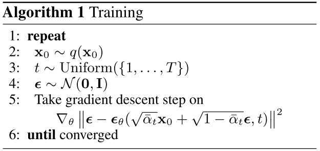
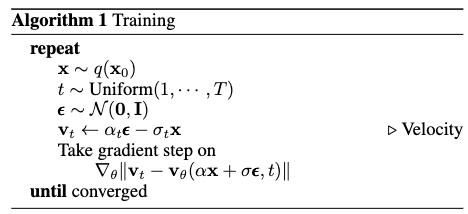
The overall DDPM training algorithm is:

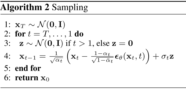
The sampling process resembles Langevin dynamics, with \(\pmb{\epsilon}_\theta\) serving as the learned gradient of the data density.

Velocity prediction

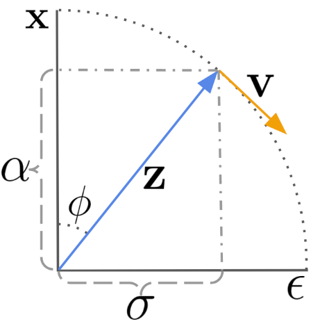
Salimans and Ho⁶ propose to parameterize the diffusion velocity by predicting \(\mathbf{v} \equiv \alpha_t \epsilon - \sigma_t \mathbf{x}\), which gives \(\hat{\mathbf{x}} = \alpha_t \mathbf{z}_t - \sigma_t \hat{\mathbf{x}}_\theta (\mathbf{z}_t)\).

Let \(\phi_t = \arctan (\sigma_t / \alpha_t)\). Assuming a variance-preserving diffusion process, we have \(\alpha_\phi = \cos (\phi)\), \(\sigma_\phi = \sin (\phi)\), and hence \(\mathbf{z}_\phi = \cos (\phi) \mathbf{x} + \sin (\phi) \epsilon\).

The velocity of \(\mathbf{z}_\phi\) is then defined as:

\[\begin{align} \mathbf{v}_\phi &{}\equiv \frac{d \mathbf{z}_\phi}{d \phi} \\ &{}= \frac{d \cos (\phi)}{d \phi} \mathbf{x} + \frac{d \sin (\phi)}{d \phi} \epsilon \\ &{}= \cos (\phi) \epsilon - \sin (\phi) \mathbf{x} \end{align}\]

By rearranging the $\epsilon$, $\mathbf{x}$, $\mathbf{v}$, we then get:

\[\begin{align} \sin (\phi) \mathbf{x} &{}= \cos(\phi) \epsilon - \mathbf{v}_\phi \\ &{}= \frac{\cos(\phi)}{\sin(\phi)} (\mathbf{z} - \cos(\phi) \mathbf{x}) - \mathbf{v}_\phi \\ \sin^2(\phi) \mathbf{x} &{}= \cos(\phi) \mathbf{z} - \cos^2(\phi)\mathbf{x} - \sin (\phi) \mathbf{v}_\phi \\ (\sin^2(\phi) + \cos^2(\phi))\mathbf{x} &{}= \mathbf{x} = \cos(\phi) \mathbf{z} - \sin (\phi) \mathbf{v}_\phi \end{align}\]

We also obtain \(\epsilon = \sin (\phi) \mathbf{z}_\phi + \cos (\phi)\mathbf{v}_\phi\).

The predicted velocity is defined as:

\[\begin{align} \hat{v}_\theta (\mathbf{z}_\phi) \equiv \cos(\phi) \hat{\epsilon}_\theta (\mathbf{z}_\phi) - \sin (\phi) \hat{\mathbf{x}}_\theta (\mathbf{z}_\phi) \end{align}\]

where \(\hat{\epsilon}_\theta (\mathbf{z}_\phi) = (\mathbf{z}_\phi - \cos(\phi)\hat{\mathbf{x}}_\theta (\mathbf{z}_\phi) ) / \sin(\phi)\).

The following algorithm illustrates the complete training process:

Conditional Generation

Conditional generation can be achieved through classifier-guided or classifier-free methods. The key distinction lies in whether an auxiliary classifier is required to steer the sampling process.

Classifier Guidance

Dhariwal and Nichol⁷ train a classifier \(f_\phi (y \vert \mathbf{x}_t,t)\) on noisy images \(\mathbf{x}_t\) and use its gradient \(\nabla_\mathbf{x} \log f_\phi (y \vert \mathbf{x}_t)\) to steer the sampling process toward a desired condition $y$ (e.g., a target class label).

Given a Gaussian \(\mathbf{x} \sim \mathcal{N}(\pmb{\mu}, \pmb{\sigma}^2\mathbf{I})\), the log derivative of the density function⁵ is:

\[\begin{align} \nabla_\mathbf{x} \log p(\mathbf{x}) &{}= \nabla_\mathbf{x} \Big( - \frac{1}{s\sigma^2} (\mathbf{x} - \pmb{\mu})^2 \Big) \\ &{}= -\frac{\mathbf{x} - \pmb{\mu}}{\pmb{\sigma}^2} \\ &{}= -\frac{\pmb{\epsilon}}{\pmb{\sigma}} \qquad \qquad\qquad \text{with}\qquad\pmb{\epsilon} \sim \mathcal{N}(\mathbf{0}, \mathbf{1}) \end{align}\]

Given Eq.\(\eqref{noise_process}\), we have:

\[\begin{align} \nabla_{\mathbf{x}_t} \log q(\mathbf{x}_t) &{}= \mathbb{E}_{q(\mathbf{x}_0)} \Big[ \nabla_{\mathbf{x}_t} q(\mathbf{x}_t \vert \mathbf{x}_0) \Big] \\ &{}= \mathbb{E}_{q(\mathbf{x}_0)} \Big[ -\frac{\pmb{\epsilon}_\theta(\mathbf{x}_t, t)}{\sqrt{1-\bar{\alpha}_t}} \Big] \\ &{}= -\frac{\pmb{\epsilon}_\theta(\mathbf{x}_t, t)}{\sqrt{1-\bar{\alpha}_t}} \end{align}\]

The score function for the joint distribution \(q (\mathbf{x}_t, y)\) is:

\[\begin{align} \nabla_{\mathbf{x}_t} \log q (\mathbf{x}_t, y) &{}= \nabla_{\mathbf{x}_t} \log q (\mathbf{x}_t) + \nabla_{\mathbf{x}_t} \log q (y \vert \mathbf{x}_t) \\ &{}\approx - \frac{1}{\sqrt{1-\bar{\alpha}_t}} \pmb{\epsilon} (\mathbf{x}_t, t) + \nabla_{\mathbf{x}_t} \log f_\phi (y \vert \mathbf{x}_t) \\ &{}= - \frac{1}{\sqrt{1-\bar{\alpha}_t}} \big( \pmb{\epsilon}_\theta (\mathbf{x}_t, t) - \sqrt{1 - \bar{\alpha}_t} \nabla_{\mathbf{x}_t} \log f_\phi (y \vert \mathbf{x}_t) \big) \end{align}\]

The classifier-guided predictor \(\bar{\pmb{\epsilon}}_\theta\) achieves a truncation-like effect by sampling in the direction of the classifier gradient:

\[\begin{align} \bar{\pmb{\epsilon}}_\theta (\mathbf{x}_t, t) = \pmb{\epsilon}_\theta (\mathbf{x}_t, t) - \sqrt{1-\bar{\alpha}_t} \nabla_{\mathbf{x}_t} \log f_\phi (y \vert \mathbf{x}_t) \end{align}\]

Dhariwal and Nichol⁷ introduce a guidance scale $w$ to control the strength of the shifted gradient:

\[\begin{align} \bar{\pmb{\epsilon}}_\theta (\mathbf{x}_t, t) = \pmb{\epsilon}_\theta (\mathbf{x}_t, t) - \sqrt{1-\bar{\alpha}_t} \nabla_{\mathbf{x}_t} {\color{red} w} \log f_\phi (y \vert \mathbf{x}_t) \label{classifier_guidance} \end{align}\]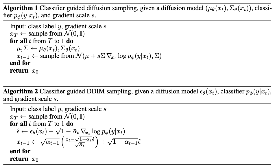

Classifier-Free Guidance

Classifier guidance introduces an auxiliary classifier and thus complicates the training pipeline. A natural question is whether we can achieve conditional generation without any explicit classifier \(f_\phi\). Ho and Salimans⁸ propose to combine the score estimates of a conditional diffusion model \(p_\theta (\mathbf{x}\vert y)\) and a jointly trained unconditional model \(p_\theta (\mathbf{x})\) within a single network.

Specifically, during training of the conditional model \(p_\theta (\mathbf{x}\vert y)\) parameterized by \(\pmb{\epsilon}_\theta (\mathbf{x}_t, t, y)\), the condition is randomly dropped by setting $y=\emptyset$, yielding \(\pmb{\epsilon}_\theta (\mathbf{x}_t, t) = \pmb{\epsilon}_\theta (\mathbf{x}_t, t, \emptyset)\).

The gradient of an implicit classifier can be formulated with the difference between conditional and unconditional classifiers:

\[\begin{align} \nabla_{\mathbf{x}_t} \log f_\phi (y \vert \mathbf{x}_t) &{} = \nabla_{\mathbf{x}_t} \log p (\mathbf{x}_t \vert y) - \nabla_{\mathbf{x}_t} \log p (\mathbf{x}_t) \\ &{}= - \frac{1}{\sqrt{1-\bar{\alpha}_t}} \big( \pmb{\epsilon}_\theta (\mathbf{x}_t, t, y) - \pmb{\epsilon}_\theta (\mathbf{x}_t, t, y=\emptyset) \big) \end{align}\]

Plugging into the Eq.\(\eqref{classifier_guidance}\), the score estimator will be:

\[\begin{align} \bar{\pmb{\epsilon}}_\theta (\mathbf{x}_t, t) &{} = \pmb{\epsilon}_\theta (\mathbf{x}_t, t) - \sqrt{1-\bar{\alpha}_t} \nabla_{\mathbf{x}_t} w \log f_\phi (y \vert \mathbf{x}_t) \\ &{}= \pmb{\epsilon}_\theta (\mathbf{x}_t, t, y) - w \Big( \pmb{\epsilon}_\theta (\mathbf{x}_t, t, y) - \pmb{\epsilon}_\theta (\mathbf{x}_t, t, y=\emptyset) \Big)\\ &{}= (w+1) \pmb{\epsilon}_\theta (\mathbf{x}_t, t, y) - w \cdot \pmb{\epsilon}_\theta (\mathbf{x}_t, t, y=\emptyset) \end{align}\]

---

Categorical Diffusion (Discrete)

Gaussian diffusion operates in continuous state spaces (e.g., real-valued image and waveform data). While some works apply Gaussian diffusion to categorical data by relaxing or embedding discrete tokens into continuous spaces, a more principled approach is categorical diffusion, which directly corrupts discrete data such as language tokens in their native state space.

Sohl-Dickstein et al.¹ first introduced diffusion models with discrete state spaces over binary random variables. Hoogeboom et al.⁹ extended the model class to categorical random variables with transition matrices characterized by uniform transition probabilities. Austin et al.¹⁰ introduced discrete denoising diffusion probabilistic models (D3PM) by more generally extending the state corruption process.

Discrete Diffusion (D3PM)

For scalar discrete random variables with $K$ categories \(x_t, x_{t-1} \in \{1,\cdots, K\}\), the forward transition probability can be represented by matrices: \([\mathbf{Q}_t]_{ij} = q (x_t = j \vert x_{t-1}=i)\).

Denoting the one-hot encoding of $x$ as the row vector $\mathbf{x}$, and writing $\text{Cat} (\mathbf{x}; \mathbf{p})$ for the categorical distribution over one-hot row vector $\mathbf{x}$ with probability vector $\mathbf{p}$, we can write:

\[\begin{align} q(\mathbf{x}_t \vert \mathbf{x}_{t-1}) = \text{Cat} (\mathbf{x}_t; \mathbf{p}=\mathbf{x}_{t-1}\mathbf{Q}_t) \end{align}\]

The term \(\mathbf{x}_{t-1}\mathbf{Q}_t\) is a row-vector–matrix product. $\mathbf{Q}$ is assumed to apply independently to each pixel or token, so $q$ factorizes over spatial/sequential dimensions. We therefore write \(q(\mathbf{x}_t \vert \mathbf{x}_{t-1})\) with respect to a single element.

Discrete state spaces

Starting from \(\mathbf{x}_0\), the $t$-step marginal at time $t$ is:

\[\begin{align} q(\mathbf{x}_t \vert \mathbf{x}_0) = \text{Cat} (\mathbf{x}_t; \mathbf{p}=\mathbf{x}_0 \mathbf{\overline{Q}}_t) \quad \quad \text{with} \quad\quad \mathbf{\overline{Q}}_t= \prod_{i=1}^t\mathbf{Q}_i \end{align}\]

The posterior is:

\[\begin{align} q(\mathbf{x}_{t-1} \vert \mathbf{x}_t, \mathbf{x}_0) &{}= \frac{q(\mathbf{x}_t \vert \mathbf{x}_{t-1}, \mathbf{x}_0) q(\mathbf{x}_{t-1}\vert \mathbf{x}_0)}{q(\mathbf{x}_{t}\vert \mathbf{x}_0)} \qquad\qquad\qquad \text{Markov property}\\ &{}= \frac{q(\mathbf{x}_t \vert \mathbf{x}_{t-1}) q(\mathbf{x}_{t-1}\vert \mathbf{x}_0)}{q(\mathbf{x}_{t}\vert \mathbf{x}_0)} \\ &{}=\text{Cat} (\mathbf{x}_t; \mathbf{p}= \frac{\mathbf{x}_t \mathbf{Q}_t^\top \odot \mathbf{x}_0 \mathbf{\overline{Q}}_{t-1}}{\mathbf{x}_0 \mathbf{\overline{Q}}_{t} \mathbf{x}_t^\top} ) \end{align}\]

Assuming the reverse process \(p_\theta (\mathbf{x}_{t-1} \vert \mathbf{x}_t)\) factorizes as conditionally independent over all elements, the KL divergence between $q$ and \(p_\theta\) decomposes into a sum over all values of each random variable.

Forward Markov transition matrices

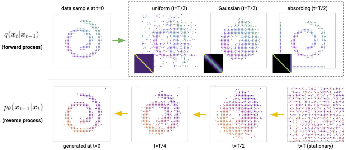
1. Uniform⁹. Given \(\beta_t \in [0,1]\), the transition matrix is \(\mathbf{Q}_t = (1-\beta_t)\mathbf{I} + \frac{\beta_t}{K} \mathbb{1}\mathbb{1}^\top\).
2. Absorbing state. The transition matrix includes an absorbing state ([MASK]): each token either stays unchanged or transitions to [MASK] with probability \(\beta_t\), inspired by BERT’s masking strategy. For images, grey pixels serve as the absorbing token.
3. Discretized Gaussian. Hoogeboom et al.⁹ use a discretized, truncated Gaussian for ordinal data such as images.
4. Token embedding distance. Hoogeboom et al.⁹ also use embedding-space similarity to guide the forward process, making transitions more frequent between tokens with similar embeddings while preserving a uniform stationary distribution.

Training

\[\begin{align} \mathcal{L}_\lambda = \mathcal{L}_{\text{vlb}} + \lambda \mathbb{E}_{q(\mathbf{x}_0}\mathbb{E}_{q(\mathbf{x}_t \vert \mathbf{x}_0)} [- \log \tilde{p}_\theta (\mathbf{x}_0 \vert \mathbf{x}_t)] \end{align}\]

BERT is a one-step diffusion model. Consider a one-step diffusion process in which \(q(\mathbf{x}_1 \vert \mathbf{x}_0)\) replaces 10% of tokens with [MASK] and 5% uniformly at random. We have:

\[\begin{align} \mathcal{L}_\text{vlb} - \mathcal{L}_\text{T} &{}= - \mathbb{E}_{q(\mathbf{x}_1 \vert \mathbf{x}_0)} [\log p_\theta (\mathbf{x}_0 \vert \mathbf{x}_1)] \\ &{}= \mathcal{L}_\text{BERT} \end{align}\]

---

Autoregressive models are (discrete) diffusion models. Consider a diffusion process that deterministically masks tokens one by one in a sequence of length $T$:

\[\begin{align} q([\textbf{x}_t]_i \vert \textbf{x}_0) =\left\{ \begin{array}{ll} [\textbf{x}_0]_i \qquad \text{if}\quad i<T-t\\ \text{[MASK]} \quad\text{otherwise} \end{array} \right. \end{align}\]

For the position $i \neq T-t$, the KL divergence

\[\begin{align} D_\text{KL}(q([\mathbf{x}_{t-1}]_i \vert \mathbf{x}_t, \mathbf{x}_0) \parallel p_\theta([\mathbf{x}_{t-1}]_i \vert\mathbf{x}_t)) \rightarrow 0 \end{align}\]

Therefore, the KL divergence is computed over the tokens at position $i$, which is exactly the standard cross entropy loss for an autoregressive model.

\[\begin{align} D_\text{KL}(q([\mathbf{x}_{t-1}]_i \vert \mathbf{x}_t, \mathbf{x}_0) \parallel p_\theta([\mathbf{x}_{t-1}]_i \vert\mathbf{x}_t)) &= q([\mathbf{x}_{t-1}]_i \vert \mathbf{x}_t, \mathbf{x}_0) \cdot \log \frac{q([\mathbf{x}_{t-1}]_i \vert \mathbf{x}_t, \mathbf{x}_0)}{p_\theta([\mathbf{x}_{t-1}]_i \vert\mathbf{x}_t)} \\ &=-p_\theta([\mathbf{x}_0]_i \vert\mathbf{x}_t) \\ &= -p_\theta(x_{t-1}\vert x_{>t}) \end{align}\]

---

(Generative) Masked Language Models are diffusion models. Generative MLMs¹¹¹² produce text by iteratively unmasking a sequence of [MASK] tokens.

References