Efficient Distributed Training: From DP to ZeRO and FlashAttention
Training billion-parameter models on a single GPU is no longer feasible—both memory and compute demands exceed what any single device can provide. The solution is parallelism, but choosing the right parallelism strategy (and combining them) is itself a non-trivial engineering problem. Data parallelism replicates the model but partitions data; tensor parallelism slices individual operators across devices; pipeline parallelism assigns different layers to different GPUs; and sequence parallelism handles the non-tensor-parallel regions. In practice, large-scale training combines all of these into a multi-dimensional parallel strategy.
This post covers the core parallelism methods—Data Parallelism, Megatron-style Tensor Parallelism, GPipe/PipeDream Pipeline Parallelism, and Sequence Parallelism—along with memory optimization techniques including ZeRO, PyTorch FSDP, mixed precision training, activation recomputation, and FlashAttention. For each method, we provide the key formulations, trade-offs, and reference implementations that practitioners need to make informed decisions when scaling training.
Training Parallelism
Data Parallelism
Data Parallelism (DP) replicates the full model on each device and partitions the mini-batch across them. Each device executes forward and backward passes on its data shard independently, then gradients are averaged via all-reduce before the synchronized weight update. DP is simple to implement and scales well when the model fits in a single GPU’s memory.
Model Parallelism (Tensor Parallelism)
Tensor-level Model Parallelism (TP)1 distributes individual operators across devices, enabling models too large for a single GPU. Megatron-LM pioneered this approach for transformers.
MLP Block
Consider the standard MLP within a transformer:
\[Y = \text{GeLU}(XA), \qquad Z = \text{Dropout}(YB)\]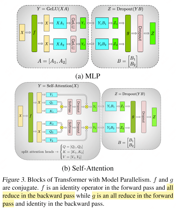
TP splits $A$ along columns: \(A = [A_1, A_2]\). Since GeLU is element-wise, it can be applied independently to each partition:
\[[Y_1, Y_2] = [\text{GeLU}(XA_1), \text{GeLU}(XA_2)]\]Matrix $B$ is then split along rows, allowing direct consumption of the GeLU outputs without inter-device communication until the final all-reduce.
Self-Attention Block
For self-attention:
\[\text{Attention}(X,Q,K,V) = \text{softmax}\!\left(\frac{(XQ)(XK)^\top}{\sqrt{d_k}}\right) XV\]TP partitions the $Q$, $K$, $V$ projection matrices along columns so that each attention head resides on a single GPU. The output projection is split along rows. This yields an efficient design requiring only two all-reduce operations per transformer layer (one in forward, one in backward).
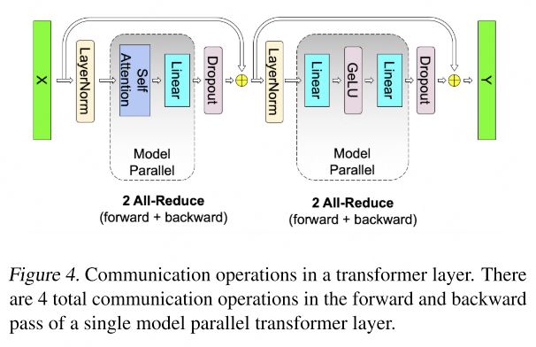
Non-parallel components: Dropout, layer normalization, and residual connections are replicated (not split) across GPUs. Each GPU maintains a duplicate of the LayerNorm parameters, allowing these operations to proceed locally without communication.
Pipeline Parallelism
Pipeline Parallelism (PP)234 assigns consecutive groups of layers to different devices, with data flowing through them sequentially as micro-batches.
GPipe
GPipe2 splits the mini-batch into $m$ micro-batches that flow through $p$ pipeline stages simultaneously.
Pipeline bubble: The unavoidable idle time at the start and end of each batch. With $p$ stages and $m$ micro-batches:
\[\text{Bubble fraction} = \frac{p - 1}{m + p - 1}\]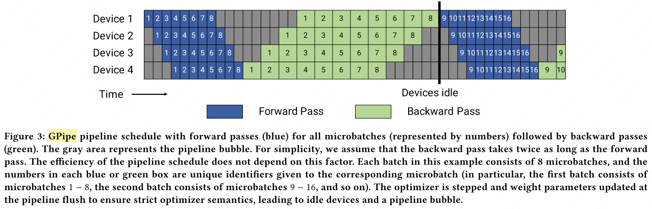
When $m \gg p$, the bubble overhead becomes negligible.
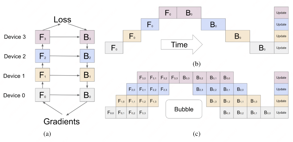
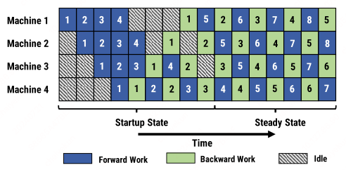
PipeDream (1F1B)
PipeDream3 introduces the one-forward-one-backward (1F1B) schedule: each device immediately starts the backward pass for a micro-batch as soon as its forward pass completes. This interleaving ensures no GPU sits idle during steady state.
With interleaved scheduling, each device handles $v$ model chunks (multiple non-contiguous stages), reducing per-micro-batch latency by $1/v$ and shrinking the bubble to:
\[\text{Bubble fraction} = \frac{1}{v} \cdot \frac{p - 1}{m + p - 1}\]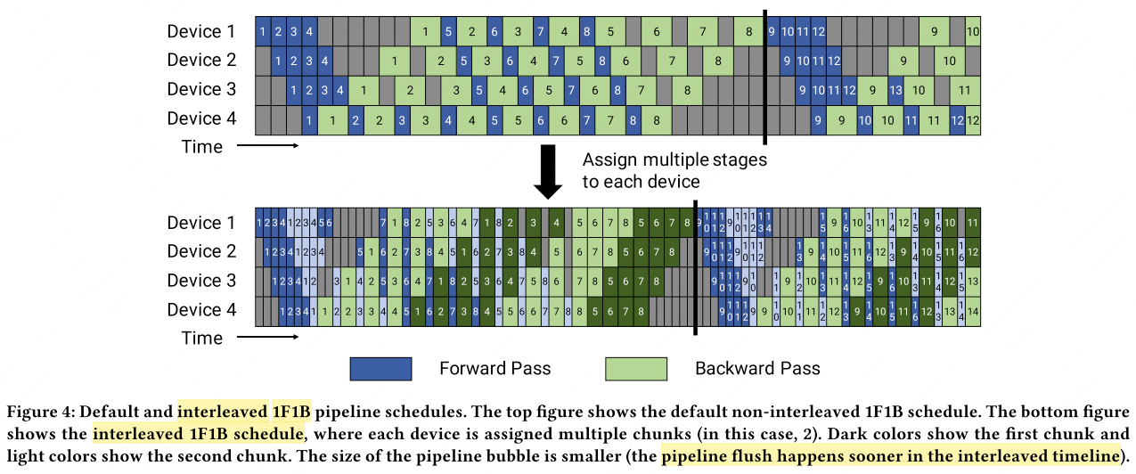
Sequence Parallelism
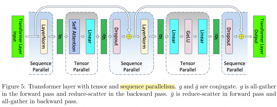
Sequence Parallelism (SP)5 targets the non-tensor-parallel regions of a transformer (LayerNorm, dropout, residual connections), which are independent along the sequence dimension.
The standard non-parallel block:
\[\begin{align} Y &= \text{LayerNorm}(X), \\ Z &= \text{GeLU}(YA), \\ W &= ZB, \\ V &= \text{Dropout}(W) \end{align}\]SP splits $X$ along the sequence dimension: \(X = [X_1^s, X_2^s]\). After LayerNorm (sequence-parallel), an all-gather provides the full $Y$ for the TP region. After the TP GEMM, reduce-scatter returns to sequence-parallel sharding:
\[\begin{align} [Y_1^s, Y_2^s] &= \text{LayerNorm}([X_1^s, X_2^s]), \\ Y &= g(Y_1^s, Y_2^s), \\ [Z_1^h, Z_2^h] &= [\text{GeLU}(YA_1^c),\; \text{GeLU}(YA_2^c)], \\ W_1 &= Z_1^h B_1^r, \quad W_2 = Z_2^h B_2^r, \\ [W_1^s, W_2^s] &= \bar{g}(W_1, W_2), \\ [V_1^s, V_2^s] &= [\text{Dropout}(W_1^s),\; \text{Dropout}(W_2^s)] \end{align}\]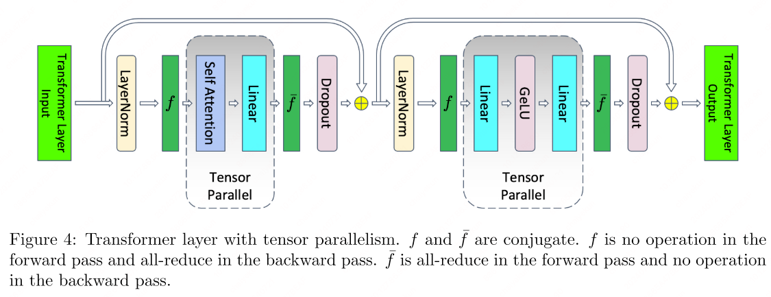
SP replaces the all-reduce in TP with all-gather (forward) and reduce-scatter (backward), keeping total communication volume constant while eliminating activation memory redundancy in non-TP regions.
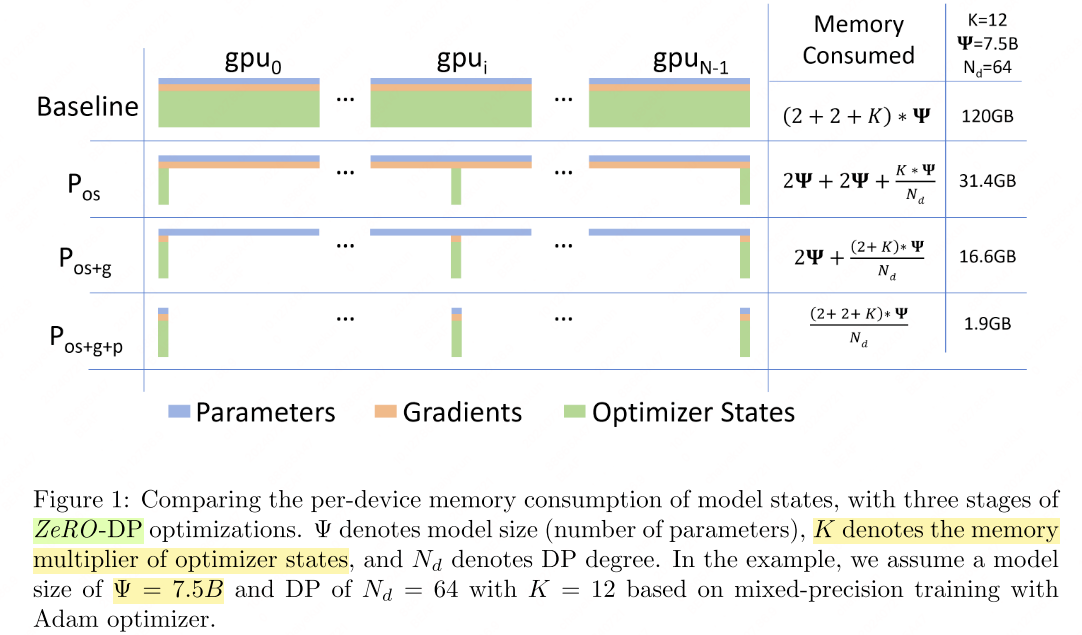
ZeRO: Memory-Efficient Optimizer
Zero Redundancy Optimizer (ZeRO)6 eliminates memory redundancy across DP ranks by partitioning (instead of replicating) model states. ZeRO has three progressive stages:
- \(P_\text{os}\): Partition optimizer states only.
- \(P_\text{os+g}\): Additionally partition gradients.
- \(P_\text{os+g+p}\): Additionally partition parameters.
See DeepSpeed ZeRO tutorial for implementation details.
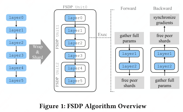
PyTorch FSDP
Fully Sharded Data Parallel (FSDP)7 shards model parameters, gradients, and optimizer states across devices. During forward/backward, only one shard is materialized (unsharded) at a time, keeping peak memory proportional to a single shard.
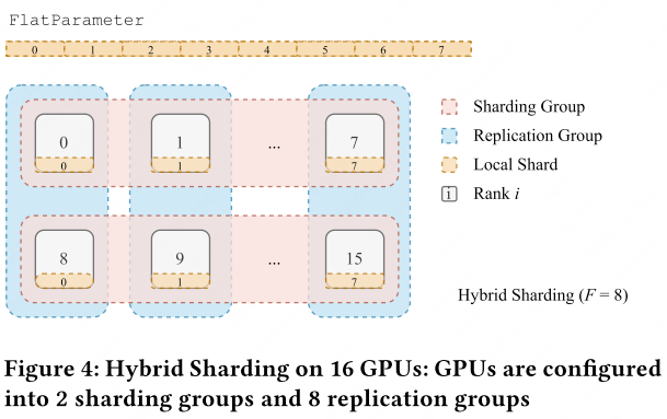
FSDP uses a sharding factor $F$:
- $F = 1$: equivalent to standard DP (all-reduce on gradients).
- $F = W$ (world size): full sharding—each device holds $1/W$ of the model.
- $1 < F < W$: hybrid sharding.
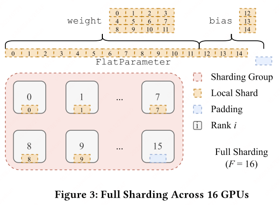
Sharding strategy (flatten-concat-chunk): All parameters within an FSDP unit are flattened into a single contiguous FlatParameter, padded if necessary for divisibility by $F$, then chunked evenly across ranks.
Mixed Precision Training
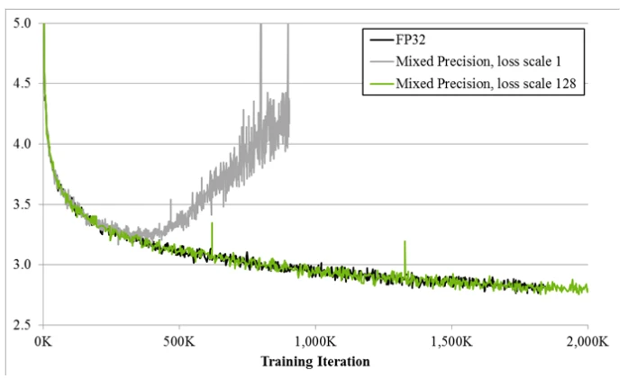
Mixed precision89 executes most operations in FP16 (or BF16) for speed, while maintaining an FP32 master copy of weights for numerical stability.
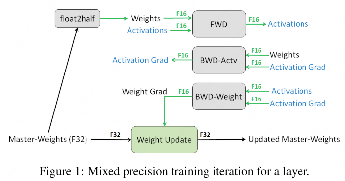
Training procedure:
- Maintain FP32 master weights.
- Each iteration: cast to FP16 → forward → scale loss by $S$ → backward → unscale gradients by $1/S$ → update FP32 master weights.
Dynamic Loss Scaling
Start with a large scaling factor $S$. If no overflow occurs for $N$ iterations, increase $S$. If overflow is detected, skip the update and decrease $S$.
1
2
3
4
5
6
7
8
9
10
11
12
13
 model = Net().cuda()
optimizer = optim.SGD(model.parameters(), ...)
scaler = GradScaler()

for epoch in epochs:
    for input, target in data:
        optimizer.zero_grad()
        with autocast(device_type='cuda', dtype=torch.float16):
            output = model(input)
            loss = loss_fn(output, target)
        scaler.scale(loss).backward()
        scaler.step(optimizer)
        scaler.update()
AMP Optimization Levels (NVIDIA Apex)
| Level | Description | Weights | Loss Scaling |
|---|---|---|---|
| O0 | Pure FP32 | FP32 | None |
| O1 | Mixed precision (recommended) | FP32, ops auto-cast | Dynamic |
| O2 | Almost FP16 | FP16 + FP32 master copy | Dynamic |
| O3 | Pure FP16 (speed baseline) | FP16 | None |
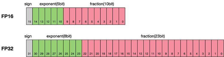
Floating-Point Formats
| Format | Exponent | Mantissa | Range | Use Case |
|---|---|---|---|---|
| FP32 | 8 bits | 23 bits | Wide | Master weights, accumulation |
| FP16 | 5 bits | 10 bits | Limited | Forward/backward compute |
| BF16 | 8 bits | 7 bits | Same as FP32 | Preferred for training stability |
| FP8 | 4-5 bits | 2-3 bits | Narrow | Emerging for inference/training |
Memory-Efficient Techniques
CPU Offload
When GPU memory is exhausted, model states (optimizer states, parameters) can be offloaded to CPU memory and fetched back on demand. ZeRO-Offload and ZeRO-Infinity implement this strategy.
Activation Recomputation
Instead of storing all intermediate activations for backpropagation, selective activation recomputation stores only a subset (e.g., activations at layer boundaries) and recomputes the rest during the backward pass. This trades compute for memory, typically with minimal wall-clock overhead.
FlashAttention
FlashAttention10 reduces HBM (High Bandwidth Memory) accesses by tiling the attention computation into SRAM-sized blocks, avoiding materialization of the full $N \times N$ attention matrix.
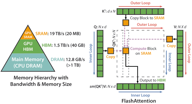
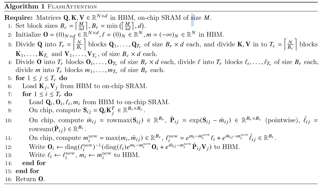
FlashAttention v1 tiles K/V in the outer loop and Q in the inner loop; v2 reverses this to reduce SRAM visits. The result is exact attention (not an approximation) with $O(N)$ memory instead of $O(N^2)$.
References
-
Shoeybi, M., et al. Megatron-LM: Training Multi-Billion Parameter Language Models Using Model Parallelism. arXiv:1909.08053, 2019. ↩
-
Huang, Y., et al. GPipe: Easy Scaling with Micro-Batch Pipeline Parallelism. NeurIPS 2019. ↩ ↩2
-
Harlap, A., et al. PipeDream: Fast and Efficient Pipeline Parallel DNN Training. SOSP 2019. ↩ ↩2
-
Narayanan, D., et al. Efficient Large-Scale Language Model Training on GPU Clusters Using Megatron-LM. SC 2021. ↩
-
Korthikanti, V.A., et al. Reducing Activation Recomputation in Large Transformer Models. MLSys 2023. ↩
-
Rajbhandari, S., et al. ZeRO: Memory Optimizations Toward Training Trillion Parameter Models. SC 2020. ↩
-
Zhao, Y., et al. PyTorch FSDP: Experiences on Scaling Fully Sharded Data Parallel. arXiv:2304.11277, 2023. ↩
-
NVIDIA. Training with Mixed Precision. ↩
-
Micikevicius, P., et al. Mixed Precision Training. ICLR 2018. ↩
-
Dao, T., et al. FlashAttention: Fast and Memory-Efficient Exact Attention with IO-Awareness. NeurIPS 2022. ↩
Related Posts