Normalization in Neural Networks: BN, LN, RMSNorm, and Beyond
Normalization is one of those techniques that every practitioner uses daily yet few fully appreciate why it works so well. The original Batch Normalization paper attributed its effectiveness to reducing “internal covariate shift”—but later work showed that explanation is likely wrong, and the real benefit is a smoother optimization landscape. Meanwhile, the landscape of normalization methods has diversified considerably: Layer Norm replaced BatchNorm for sequence models, RMSNorm simplified it further for LLMs (now the default in Llama, Gemma, and most modern architectures), and Group Norm solved the small-batch problem in detection and segmentation.
This post walks through the major normalization variants—BatchNorm, LayerNorm, RMSNorm, InstanceNorm, GroupNorm, and Switchable Norm—with precise formulations, reference implementations, and a unified comparison of which axes each method normalizes over. The goal is to give practitioners a clear mental model for choosing the right normalization in any context: CNNs, RNNs, Transformers, or style transfer.
Data Preprocessing
Standard feature normalization: subtract the mean and scale by the standard deviation.
\[\hat{x}_i^n = \frac{x_i^n - \text{mean}(x_i)}{\text{std}(x_i)}\]Other common preprocessing steps include PCA (projecting onto top principal components for decorrelation and dimensionality reduction) and whitening (PCA followed by per-dimension scaling to unit variance).
Batch Normalization
Motivation: During training, the distribution of each layer’s inputs shifts as preceding layers’ parameters change—a phenomenon originally termed internal covariate shift. This slows convergence by requiring lower learning rates and careful initialization, and makes it difficult to train networks with saturating nonlinearities.
Solution: Batch Normalization (BN)1 normalizes activations using mini-batch statistics.
- Learnable parameters $\gamma$ (scale) and $\beta$ (shift) restore representational power.
- At inference time, running averages of mean and variance (computed during training) replace mini-batch statistics.
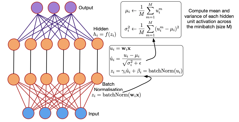
Given values of $x$ over a mini-batch \(\mathcal{B} = \{x_1, \ldots, x_m\}\):
Mini-batch mean:
\[\mu_{\mathcal{B}} \leftarrow \frac{1}{m}\sum_{i=1}^m x_i\]Mini-batch variance:
\[\sigma_{\mathcal{B}}^2 \leftarrow \frac{1}{m} \sum_{i=1}^m (x_i - \mu_{\mathcal{B}})^2\]Normalize:
\[\hat{x}_i \leftarrow \frac{x_i - \mu_{\mathcal{B}}}{\sqrt{\sigma_{\mathcal{B}}^2 + \epsilon}}\]Scale and shift:
\[y_i \leftarrow \gamma \hat{x}_i + \beta \equiv \text{BN}_{\gamma, \beta}(x_i)\]Parameters $\gamma$ and $\beta$ are learnable with size $C$ (channel dimension), initialized to ones and zeros respectively.
1
2
3
4
5
6
7
8
9
10
11
12
13
14
15
16
17
18
19
20
 class BatchNorm(nn.Module):
    def __init__(self, num_features, num_dims):
        super().__init__()
        if num_dims == 2:
            shape = (1, num_features)
        else:
            shape = (1, num_features, 1, 1)
        self.gamma = nn.Parameter(torch.ones(shape))
        self.beta = nn.Parameter(torch.zeros(shape))
        self.moving_mean = torch.zeros(shape)
        self.moving_var = torch.ones(shape)

    def forward(self, X):
        if self.moving_mean.device != X.device:
            self.moving_mean = self.moving_mean.to(X.device)
            self.moving_var = self.moving_var.to(X.device)
        Y, self.moving_mean, self.moving_var = batch_norm(
            X, self.gamma, self.beta, self.moving_mean, self.moving_var,
            eps=1e-5, momentum=0.9)
        return Y
Benefits:
- Enables higher learning rates and reduces sensitivity to weight initialization.
- Acts as a regularizer, sometimes reducing the need for dropout.
- Prevents training from getting stuck in saturated regimes of nonlinearities.
Drawbacks:
- Behaves differently at training vs. inference time.
- Degrades with very small batch sizes due to noisy statistics estimation.
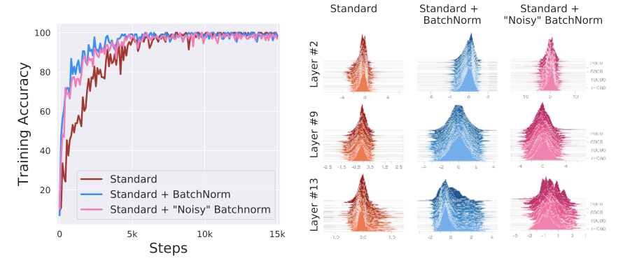
Rethinking BN (NeurIPS 2018)2: Santurkar et al. argue there is no causal link between BN’s performance gain and reduction of internal covariate shift. Their experiments inject severe covariate shift after BN—and BN still helps. The real mechanism: BN makes the optimization landscape significantly smoother, improving the Lipschitzness and effective $\beta$-smoothness of the loss function.
Layer Normalization
Motivation: BN depends on mini-batch statistics, making it unsuitable for very small batches or variable-length sequences (RNNs). It is also not straightforward to apply BN to recurrent architectures.
Solution: Layer Normalization (LN)3 computes statistics over all hidden units in the same layer:
\[\mu^l = \frac{1}{H} \sum_{i=1}^{H} a_i^l, \qquad \sigma^l = \sqrt{\frac{1}{H} \sum_{i=1}^H (a_i^l - \mu^l)^2}\]where $H$ is the number of hidden units. All hidden states in a layer share the same $\mu$ and $\sigma$, and there is no dependence on batch size (works with batch size 1).
\[y = \frac{x - \mathbb{E}[x]}{\sqrt{\text{Var}[x] + \epsilon}} \cdot \gamma + \beta\]The mean and standard deviation are computed over the last $D$ dimensions. The parameter count is $2D$ ($\gamma$ and $\beta$).
1
2
3
4
5
6
7
8
9
10
11
 class LayerNorm(nn.Module):
    def __init__(self, features, eps=1e-6):
        super().__init__()
        self.weight = nn.Parameter(torch.ones(features))
        self.bias = nn.Parameter(torch.zeros(features))
        self.eps = eps

    def forward(self, x):
        mean = x.mean(-1, keepdim=True)
        std = x.std(-1, keepdim=True)
        return self.weight * (x - mean) / (std + self.eps) + self.bias
Layer Normalization on RNNs
Given previous hidden state $\pmb{h}^{t-1}$ and current input $\pmb{x}^t$:
\[\pmb{a}^t = W_{hh}\pmb{h}^{t-1} + W_{xh}\pmb{x}^t\]Apply layer normalization:
\[\pmb{h}^t = f\!\left(\frac{\pmb{g}}{\sigma^t} \odot (\pmb{a}^t - \mu^t) + \pmb{b}\right)\]where \(\mu^t = \frac{1}{H} \sum_{i=1}^H a_i^t\) and \(\sigma^t = \sqrt{\frac{1}{H} \sum_{i=1}^H (a_i^t - \mu^t)^2}\).
BN vs. LN:
- LN: neurons in the same layer share $\mu$ and $\sigma$; different samples have different statistics.
- BN: samples in the same batch share $\mu$ and $\sigma$; different channels have different statistics.
Unlike BN, LN performs exactly the same computation at training and test time.
RMSNorm
Root Mean Square Layer Normalization (RMSNorm)4 hypothesizes that the re-scaling invariance (not the re-centering invariance) is the key reason LayerNorm works. RMSNorm drops the mean subtraction entirely and normalizes using the root mean square:
\[\bar{a}_i = \frac{a_i}{\text{RMS}(\mathbf{a})} g_i, \qquad \text{where } \text{RMS}(\mathbf{a}) = \sqrt{\frac{1}{n}\sum_{i=1}^n a_i^2}\]When the mean of summed inputs is zero, RMSNorm is exactly equal to LayerNorm. In practice, RMSNorm is cheaper to compute (no mean subtraction) and has become the default normalization in modern LLMs including Llama, Gemma, and Qwen.
1
2
3
4
5
6
7
8
9
10
11
12
13
14
15
16
17
18
19
20
21
22
23
24
25
 class RMSNorm(nn.Module):
    def __init__(self, d, p=-1., eps=1e-8, bias=False):
        super().__init__()
        self.eps = eps
        self.d = d
        self.p = p
        self.bias = bias
        self.scale = nn.Parameter(torch.ones(d))
        if self.bias:
            self.offset = nn.Parameter(torch.zeros(d))

    def forward(self, x):
        if self.p < 0. or self.p > 1.:
            norm_x = x.norm(2, dim=-1, keepdim=True)
            d_x = self.d
        else:
            partial_size = int(self.d * self.p)
            partial_x, _ = torch.split(x, [partial_size, self.d - partial_size], dim=-1)
            norm_x = partial_x.norm(2, dim=-1, keepdim=True)
            d_x = partial_size
        rms_x = norm_x * d_x ** (-1. / 2)
        x_normed = x / (rms_x + self.eps)
        if self.bias:
            return self.scale * x_normed + self.offset
        return self.scale * x_normed
Llama implementation:
1
2
3
4
5
6
7
8
9
10
11
12
 class LlamaRMSNorm(nn.Module):
    def __init__(self, hidden_size, eps=1e-6):
        super().__init__()
        self.weight = nn.Parameter(torch.ones(hidden_size))
        self.variance_epsilon = eps

    def forward(self, x):
        input_dtype = x.dtype
        x = x.to(torch.float32)
        variance = x.pow(2).mean(-1, keepdim=True)
        x = x * torch.rsqrt(variance + self.variance_epsilon)
        return self.weight * x.to(input_dtype)
Instance Normalization
Motivation: Image style transfer relies on instance-specific statistics rather than batch-level ones.
Solution: Instance Normalization (IN)5 performs per-sample, per-channel normalization and behaves identically at train and test time:
\[y_{tijk} = \frac{x_{tijk} - \mu_{ti}}{\sqrt{\sigma^2_{ti} + \epsilon}}\] \[\mu_{ti} = \frac{1}{HW} \sum_{l=1}^W \sum_{m=1}^H x_{tilm}, \qquad \sigma^2_{ti} = \frac{1}{HW} \sum_{l=1}^W \sum_{m=1}^H (x_{tilm} - \mu_{ti})^2\]Group Normalization
Motivation: BN’s error increases sharply when batch size becomes small due to inaccurate statistics estimation—a common scenario in object detection and segmentation.
Solution: Group Normalization (GN)6 divides channels into $G$ groups and computes mean/variance within each group:
\[S_i = \left\{k \;\middle\vert\; k_N = i_N,\; \left\lfloor \frac{k_C}{C/G} \right\rfloor = \left\lfloor \frac{i_C}{C/G} \right\rfloor \right\}\]GN computes $\mu$ and $\sigma$ along $(H, W)$ and across $C/G$ channels per group. Its computation is independent of batch size.
1
2
3
4
5
6
7
8
 def GroupNorm(x, gamma, beta, G, eps=1e-5):
    N, C, H, W = x.shape
    x = x.reshape(N, G, C // G, H, W)
    mean = x.mean(axis=(2, 3, 4), keepdims=True)
    var = x.var(axis=(2, 3, 4), keepdims=True)
    x = (x - mean) / np.sqrt(var + eps)
    x = x.reshape(N, C, H, W)
    return x * gamma + beta
Switchable Normalization
Motivation: Different tasks benefit from different normalizers (BN for classification, IN for style transfer, LN for sequences), making it cumbersome to manually select the right one.
Solution: Switchable Normalization (SN)7 combines IN, LN, and BN statistics with learned importance weights:
\[\hat{h}_{ncij} = \gamma \frac{h_{ncij} - \sum_{k \in \Omega} w_k \mu_k}{\sqrt{\sum_{k \in \Omega} w'_k \sigma_k^2 + \epsilon}} + \beta\]where $\Omega = {\text{in}, \text{ln}, \text{bn}}$ and the weights \(w_k, w'_k\) are learned end-to-end.
1
2
3
4
5
6
7
8
9
10
11
 def SwitchableNorm(x, gamma, beta, w_mean, w_var, eps=1e-5):
    mean_in = np.mean(x, axis=(2, 3), keepdims=True)
    var_in = np.var(x, axis=(2, 3), keepdims=True)
    mean_ln = np.mean(x, axis=(1, 2, 3), keepdims=True)
    var_ln = np.var(x, axis=(1, 2, 3), keepdims=True)
    mean_bn = np.mean(x, axis=(0, 2, 3), keepdims=True)
    var_bn = np.var(x, axis=(0, 2, 3), keepdims=True)
    mean = w_mean[0] * mean_in + w_mean[1] * mean_ln + w_mean[2] * mean_bn
    var = w_var[0] * var_in + w_var[1] * var_ln + w_var[2] * var_bn
    x_normalized = (x - mean) / np.sqrt(var + eps)
    return gamma * x_normalized + beta
Comparison
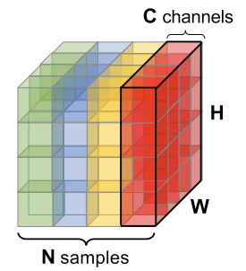
For a mini-batch tensor with shape $[N, C, H, W]$:
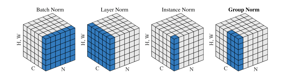
| Method | Normalizes Over | Batch-Independent | Best For |
|---|---|---|---|
| BatchNorm | $(N, H, W)$ | No | CNNs with large batches |
| LayerNorm | $(C, H, W)$ | Yes | Transformers, RNNs |
| RMSNorm | $(C, H, W)$, no mean | Yes | LLMs (Llama, Gemma, Qwen) |
| InstanceNorm | $(H, W)$ | Yes | Style transfer |
| GroupNorm | $(C/G, H, W)$ | Yes | Detection/segmentation (small batch) |
| SwitchableNorm | Learned mix of IN/LN/BN | Partially | Automatic selection |
References
-
Ioffe, S. and Szegedy, C. Batch Normalization: Accelerating Deep Network Training by Reducing Internal Covariate Shift. ICML 2015. ↩
-
Santurkar, S., Tsipras, D., Ilyas, A. and Madry, A. How Does Batch Normalization Help Optimization?. NeurIPS 2018. ↩
-
Ba, J.L., Kiros, J.R. and Hinton, G.E. Layer Normalization. arXiv:1607.06450, 2016. ↩
-
Zhang, B. and Sennrich, R. Root Mean Square Layer Normalization. NeurIPS 2019. ↩
-
Ulyanov, D., Vedaldi, A. and Lempitsky, V. Instance Normalization: The Missing Ingredient for Fast Stylization. arXiv:1607.08022, 2016. ↩
-
Wu, Y. and He, K. Group Normalization. ECCV 2018. ↩
-
Luo, P., Ren, J., Peng, Z., Zhang, R. and Li, J. Differentiable Learning-to-Normalize via Switchable Normalization. arXiv:1806.10779, 2018. ↩
Related Posts