Attention Mechanisms and the Transformer Architecture
The attention mechanism is perhaps the most consequential architectural innovation in modern deep learning. It emerged from a simple observation: compressing an entire source sentence into a single fixed-length vector is a fundamental information bottleneck. Bahdanau et al. (2014) showed that allowing the decoder to attend to all encoder hidden states—weighting them by learned alignment scores—dramatically improved machine translation, especially for long sentences. This idea of dynamic, content-dependent weighting proved so powerful that Vaswani et al. (2017) built an entire architecture around it: the Transformer, which replaced recurrence entirely with self-attention.
This post covers the progression from seq2seq to the Transformer: additive attention, the attention score function zoo, scaled dot-product and multi-head attention with complete implementations, the encoder-decoder architecture, positional encoding, and relative position representations (RPR).
Background: The Seq2Seq Bottleneck
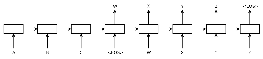
The encoder-decoder architecture1 encodes a variable-length input \((x_1, \ldots, x_T)\) into a fixed-length context vector $c$, then decodes it into the target \((y_1, \ldots, y_{T'})\):
\[p(y_1, \ldots, y_{T'} \vert x_1, \ldots, x_T) = \prod_{t=1}^{T'} p(y_t \vert c, y_1, \ldots, y_{t-1})\] \[p(y_t \vert c, y_1, \ldots, y_{t-1}) = g(y_{t-1}, s_t, c)\]Problem: The fixed-length context vector $c$ becomes a bottleneck for long sequences—the encoder must compress all information into a single vector, and performance drops sharply as input length increases2.
Attention Mechanism (Bahdanau et al., 2014)
Instead of a single context vector, the decoder attends to all encoder hidden states with a distinct context vector \(c_i\) for each target position3:
Encoder: Bidirectional RNN produces annotations \(h_j = [\overrightarrow{h}_j^\top,\, \overleftarrow{h}_j^\top]^\top\).
Decoder:
\[c_i = \sum_{j=1}^{T_x} \alpha_{ij} h_j, \qquad \alpha_{ij} = \frac{\exp(e_{ij})}{\sum_{k=1}^{T_x} \exp(e_{ik})}, \qquad e_{ij} = \text{score}(s_{i-1}, h_j)\]where $\text{score}$ is the additive (Bahdanau) alignment model:
\[\text{score}(s_t, h_i) = \mathbf{v}_a^\top \tanh(\mathbf{W}_a [s_t;\, h_i])\]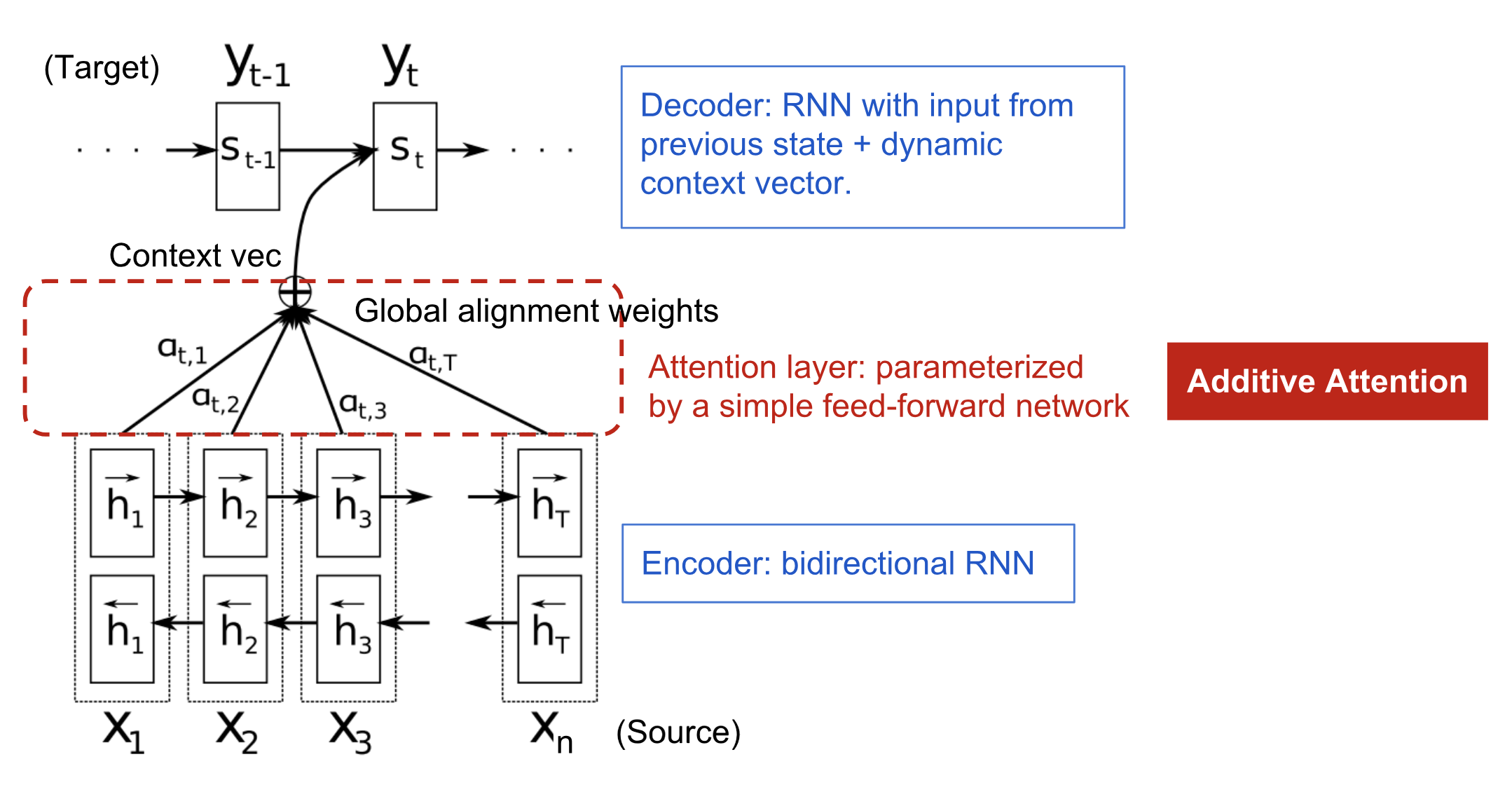
Attention Score Functions
| Type | Score Function | Reference |
|---|---|---|
| Additive (concat) | \(\mathbf{v}_a^\top \tanh(\mathbf{W}_a[\mathbf{h}_t;\, \bar{\mathbf{h}}_s])\) | Bahdanau3 |
| General | \(\mathbf{h}_t^\top \mathbf{W}_a \bar{\mathbf{h}}_s\) | Luong4 |
| Dot-product | \(\mathbf{h}_t^\top \bar{\mathbf{h}}_s\) | Luong4 |
| Scaled dot-product | \(\mathbf{h}_t^\top \bar{\mathbf{h}}_s / \sqrt{d}\) | Vaswani5 |
| Location-based | \(\text{softmax}(\mathbf{W}_a \mathbf{h}_t)\) | Luong4 |
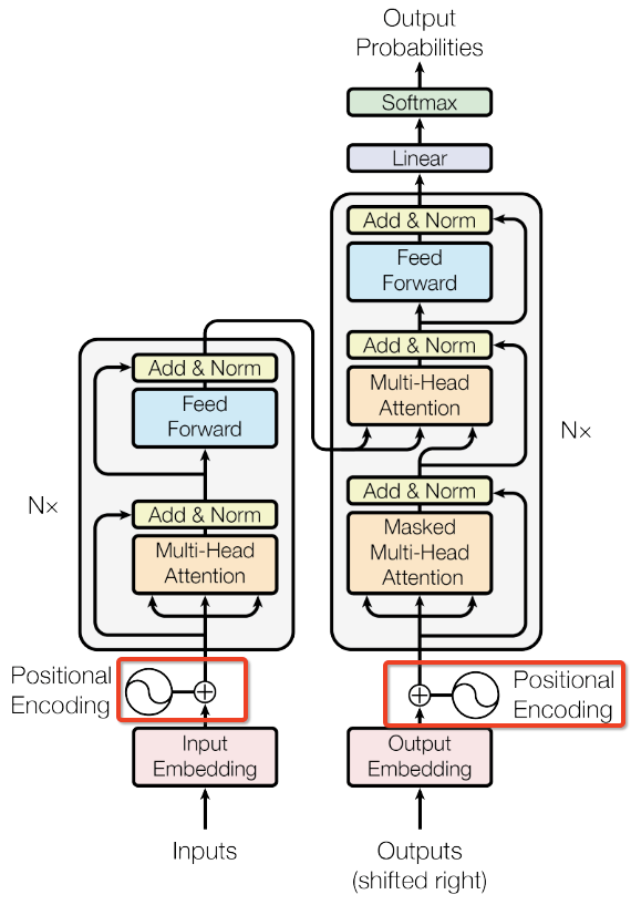
Transformer Architecture
The Transformer5 replaces recurrence entirely with stacked self-attention and point-wise feed-forward layers, connected by residual connections and layer normalization: $\text{LayerNorm}(x + \text{Sublayer}(x))$.
Encoder
$N = 6$ identical layers, each containing multi-head self-attention followed by a position-wise FFN:
1
2
3
4
5
6
7
8
9
10
 class EncoderLayer(nn.Module):
    def __init__(self, size, self_attn, feed_forward, dropout):
        super().__init__()
        self.self_attn = self_attn
        self.feed_forward = feed_forward
        self.sublayer = clones(SublayerConnection(size, dropout), 2)

    def forward(self, x, mask):
        x = self.sublayer[0](x, lambda x: self.self_attn(x, x, x, mask))
        return self.sublayer[1](x, self.feed_forward)
Decoder
$N = 6$ identical layers with an additional cross-attention sub-layer that attends to the encoder output. The first self-attention is masked to prevent attending to future positions:
1
2
3
4
5
6
7
8
9
10
11
12
 class DecoderLayer(nn.Module):
    def __init__(self, size, self_attn, src_attn, feed_forward, dropout):
        super().__init__()
        self.self_attn = self_attn
        self.src_attn = src_attn
        self.feed_forward = feed_forward
        self.sublayer = clones(SublayerConnection(size, dropout), 3)

    def forward(self, x, memory, src_mask, tgt_mask):
        x = self.sublayer[0](x, lambda x: self.self_attn(x, x, x, tgt_mask))
        x = self.sublayer[1](x, lambda x: self.src_attn(x, memory, memory, src_mask))
        return self.sublayer[2](x, self.feed_forward)
Scaled Dot-Product Attention
\[\text{Attention}(\mathbf{Q}, \mathbf{K}, \mathbf{V}) = \text{softmax}\!\left(\frac{\mathbf{Q}\mathbf{K}^\top}{\sqrt{d_k}}\right) \mathbf{V}\]Why scale by \(\sqrt{d_k}\)? For large \(d_k\), the dot products grow in magnitude (\(\text{Var}(q \cdot k) = d_k\) when \(q_i, k_i \sim \mathcal{N}(0, 1)\)), pushing softmax into saturated regions with vanishing gradients.
1
2
3
4
5
6
7
8
9
 def attention(query, key, value, mask=None, dropout=None):
    d_k = query.size(-1)
    scores = torch.matmul(query, key.transpose(-2, -1)) / math.sqrt(d_k)
    if mask is not None:
        scores = scores.masked_fill(mask == 0, -1e9)
    p_attn = F.softmax(scores, dim=-1)
    if dropout is not None:
        p_attn = dropout(p_attn)
    return torch.matmul(p_attn, value), p_attn
Multi-Head Attention
Project $\mathbf{Q}, \mathbf{K}, \mathbf{V}$ into $h$ different subspaces, compute attention in parallel, then concatenate:
\[\text{MultiHead}(\mathbf{Q}, \mathbf{K}, \mathbf{V}) = \text{Concat}(\text{head}_1, \ldots, \text{head}_h)\, W^O\] \[\text{head}_i = \text{Attention}(\mathbf{Q} W_i^Q,\, \mathbf{K} W_i^K,\, \mathbf{V} W_i^V)\]
1
2
3
4
5
6
7
8
9
10
11
12
13
14
15
16
17
18
19
 class MultiHeadedAttention(nn.Module):
    def __init__(self, h, d_model, dropout=0.1):
        super().__init__()
        assert d_model % h == 0
        self.d_k = d_model // h
        self.h = h
        self.linears = clones(nn.Linear(d_model, d_model), 4)
        self.dropout = nn.Dropout(p=dropout)

    def forward(self, query, key, value, mask=None):
        if mask is not None:
            mask = mask.unsqueeze(1)
        nbatches = query.size(0)
        query, key, value = [
            l(x).view(nbatches, -1, self.h, self.d_k).transpose(1, 2)
            for l, x in zip(self.linears, (query, key, value))]
        x, self.attn = attention(query, key, value, mask=mask, dropout=self.dropout)
        x = x.transpose(1, 2).contiguous().view(nbatches, -1, self.h * self.d_k)
        return self.linears[-1](x)
Position-wise Feed-Forward Network
\[\text{FFN}(x) = \max(0, xW_1 + b_1)W_2 + b_2\]
1
2
3
4
5
6
7
8
9
 class PositionwiseFeedForward(nn.Module):
    def __init__(self, d_model, d_ff, dropout=0.1):
        super().__init__()
        self.w_1 = nn.Linear(d_model, d_ff)
        self.w_2 = nn.Linear(d_ff, d_model)
        self.dropout = nn.Dropout(dropout)

    def forward(self, x):
        return self.w_2(self.dropout(F.relu(self.w_1(x))))
Positional Encoding
Self-attention is permutation-invariant and cannot capture sequence order. The Transformer adds sinusoidal positional encodings:
\[\text{PE}_{(\text{pos}, 2i)} = \sin\!\left(\frac{\text{pos}}{10000^{2i/d_\text{model}}}\right), \qquad \text{PE}_{(\text{pos}, 2i+1)} = \cos\!\left(\frac{\text{pos}}{10000^{2i/d_\text{model}}}\right)\]For any fixed offset $k$, \(\text{PE}_{\text{pos}+k}\) can be expressed as a linear function of \(\text{PE}_\text{pos}\), enabling the model to learn relative positions.
1
2
3
4
5
6
7
8
9
10
11
12
13
14
15
 class PositionalEncoding(nn.Module):
    def __init__(self, d_model, dropout, max_len=5000):
        super().__init__()
        self.dropout = nn.Dropout(p=dropout)
        pe = torch.zeros(max_len, d_model)
        position = torch.arange(0., max_len).unsqueeze(1)
        div_term = torch.exp(torch.arange(0., d_model, 2) * -(math.log(1e4) / d_model))
        pe[:, 0::2] = torch.sin(position * div_term)
        pe[:, 1::2] = torch.cos(position * div_term)
        pe = pe.unsqueeze(0)
        self.register_buffer('pe', pe)

    def forward(self, x):
        x = x + self.pe[:, :x.size(1)]
        return self.dropout(x)
Relative Position Representations (RPR)
Shaw et al.6 extend self-attention with learned relative position embeddings \(a_{ij}^K, a_{ij}^V\):
\[e_{ij} = \frac{x_i W^Q (x_j W^K + a_{ij}^K)^\top}{\sqrt{d_k}}, \qquad z_i = \sum_{j=1}^n \alpha_{ij}(x_j W^V + a_{ij}^V)\]Positions beyond a maximum distance $k$ are clipped:
\[a_{ij}^K = w^K_{\text{clip}(j-i, k)}, \qquad \text{clip}(x, k) = \max(-k, \min(k, x))\]This allows the model to generalize to unseen sequence lengths while keeping a bounded number of learned parameters (\(2 \times (2k+1) \times d_k\)).
References
-
Sutskever, I., Vinyals, O. and Le, Q.V. Sequence to Sequence Learning with Neural Networks. NeurIPS 2014. ↩
-
Cho, K., et al. On the Properties of Neural Machine Translation: Encoder-Decoder Approaches. SSST@EMNLP 2014. ↩
-
Bahdanau, D., Cho, K. and Bengio, Y. Neural Machine Translation by Jointly Learning to Align and Translate. ICLR 2015. ↩ ↩2
-
Luong, T., Pham, H. and Manning, C.D. Effective Approaches to Attention-based Neural Machine Translation. EMNLP 2015. ↩ ↩2 ↩3
-
Vaswani, A., et al. Attention Is All You Need. NeurIPS 2017. ↩ ↩2
-
Shaw, P., Uszkoreit, J. and Vaswani, A. Self-Attention with Relative Position Representations. NAACL 2018. ↩
Related Posts