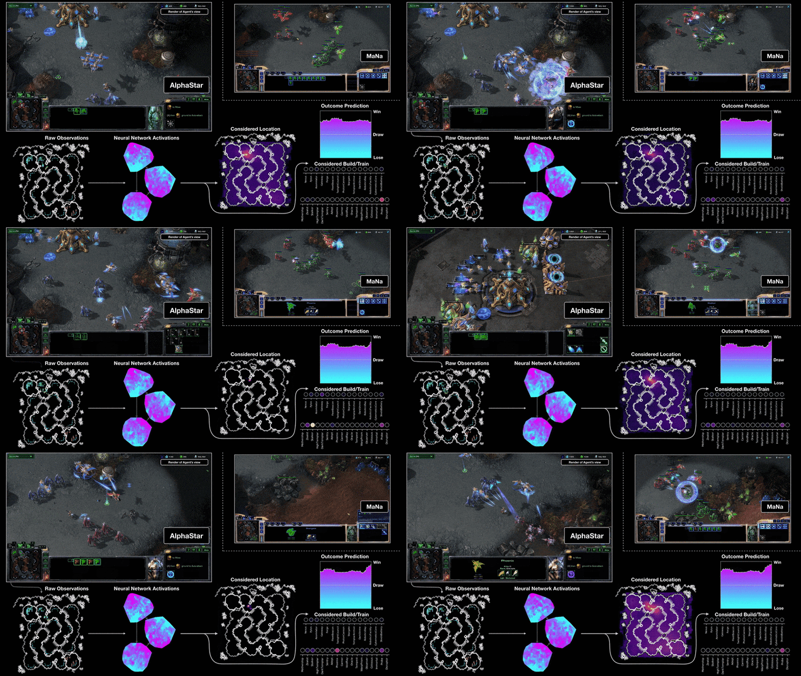
On 19 December 2018, AlphaStar has decisively beaten human player MaNa with 5-0 on StarCraft II, one of the most challenging Real-Time-Strategy (RTS) games.

How AlphaStar is trained

Imitation learning (supervised)
- AlphaStar is initially trained with imitation learning with anonymous game replays from human experts
- This offers a good initialization for neural networks
- This initial agent beats the built-in “Elite” level AI ($\approx$ human golden level)
RL
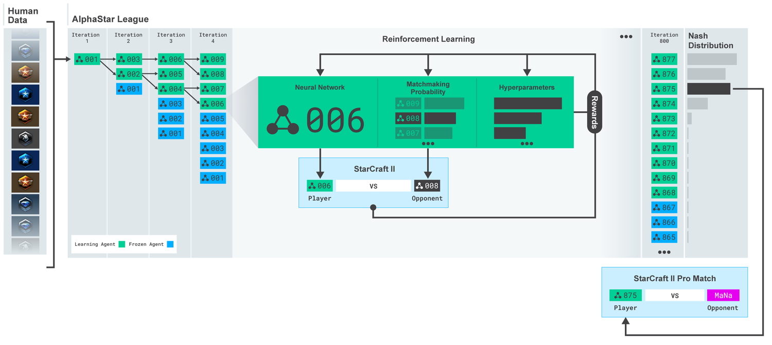
- Seed a multi-agent reinforcement learning process with a continuous league

AlphaStar League

Multi-agent RL in the presence of strategy cycles

The league contains $m$ agents and $n$ competitors
- Agent: actively learning agent, updating a policy
- Competitor: passive policy, not learning
Each agent plays games against other agents/competitors and learns by RL
- Ensuring robust performance against a wide diversity of counter-strategies
- Several mechanisms encourage diversity among the league
Agents periodically replicate into a competitor
- The new competitor is added to the league
- Ensure that agents do not forget how to defeat old selves

Agent Diversity

Each agent’s personalized objective is described by:

Matchmaking distribution over opponent to play in each game
Intrinsic reward function specifying preferences (e.g. over unit types)

Matchmaking Strategies

Prioritised Fictious Self-Play (pFSP)

Matchmaking distribution is proportional to win-rate of opponents
Encourages monotonic progress against set of competitors

Exploiters

Matchmaking distribution is uniform over individual agents
The sole goal of an exploiter is to identify the weaknesses in agents
The agents can then learn to defend against those weakness

Reinforcement Learning

Agent parameters updated by off-policy RL from replayed subsequence

Advantage Actor-Critic
V-Trace + TD($\lambda$)
Self-imitation learning
Entropy regularisation
Policy distillation

Challenges

Exploration and diversity

Solution 1: use human data to aid in exploration and to preserve strategic diversity throughout training. After initialization with SL, AlphaStar continually minimizes the KL divergence between the supervised and current policy.
Solution 2: apply pseudo-rewards to follow a strategy statistic $z$, from randomly sampled human data. The pseudo-rewards measure the edit distance between sampled and execeuted build orders; and the Hamming distances between sampled and executed cumulative statistics.
It shows that the utilzation of human data is critical in final results.

def hamming_distance(s1, s2):
	""" Return the Hamming distance between equal-length sequences """
    if len(s1)!=len(s2): raise ValueError("Non-equal length given!")
    return sum(e1!=e2 for e1,e2 in zip(s1,s2))

Supervised Learning

Three reasons for supervised learning (SL)

Provide simpler evaluation metric than multi-agent RL
- A good network architecture for SL is likely to also be good for RL
Initialization. Starting from human behaviour speeds up learning
- Initialize all policy weights $\theta = \theta^\text{SL}$
Maintain diverse exploration. Staying close to human behaviour ensures exploration of reasonable strategies
- Add $\text{KL}(\theta \vert\vert \theta^\text{SL})$ cost to RL update
- This is the solution to avoid naive exploration in micro-tactics of ground units, e.g. naively build and use air units. The agents are also penalized whenever their action probabilties differ from the supervised policy.

AlphaStar architecture

Nature AlphaStar detailed model. It uses scatter connection to combine spatial and non-spatial features.

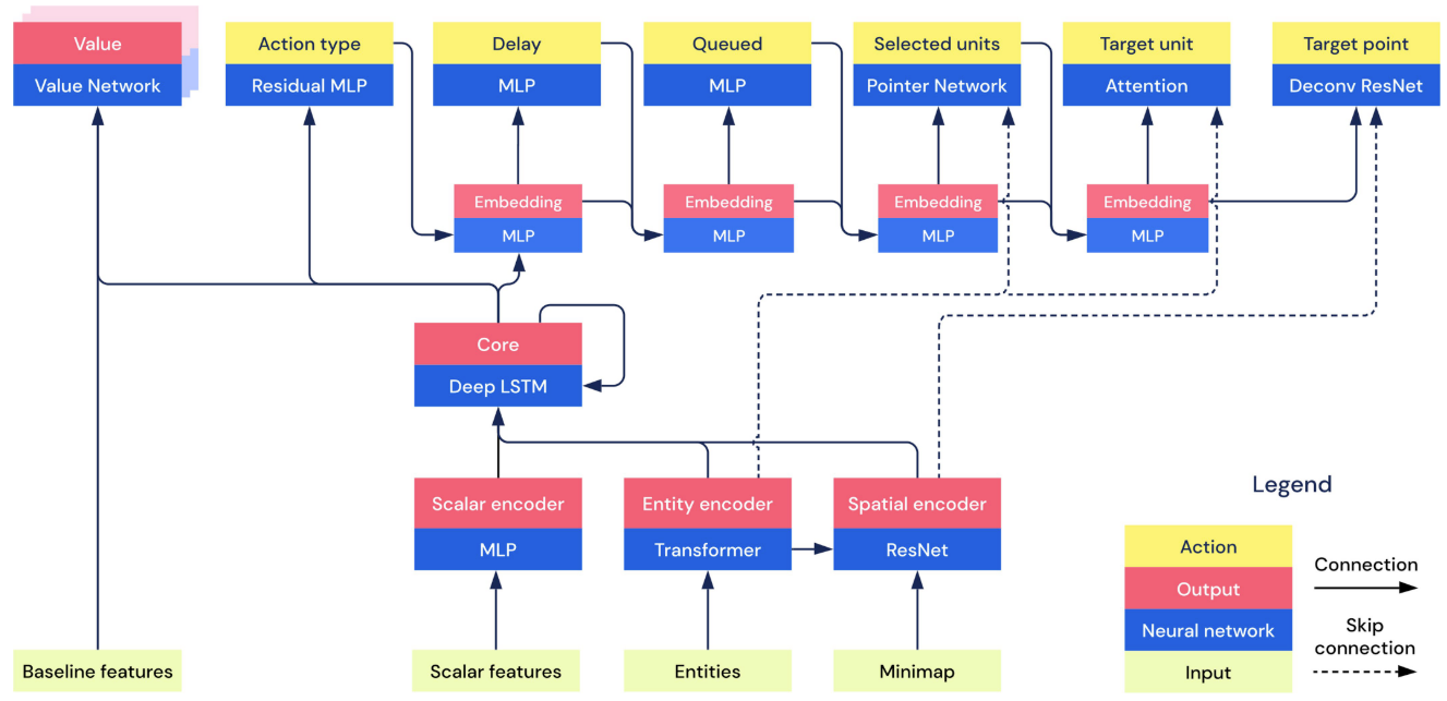
Network Inputs

prev_state: the previous LSTM state^[19]
entity_list: entities within the game
map: game map
scalar_features: player data, game statistics, build orders.
opponent_observations: opponent’s observations (only used for baselines, not for inference during play).
cumulative_score: various score metrics of the game (only used for baselines, not for inference during play). “It includes score, idle production and work time, total value of units and structure, total destroyed value of units and structures, total collected minerals and vespene, rate of minerals and vespene collection, and total spent minerals and vespene“^[19].

Encoders

Entity encoder

Input: entity_list
Output:
embedded_entity - a 1D tensor (one embedding for all entities)
entity_embeddings - one embedding for each entity, including lots of fields, involving unit_type, unit_attr, alliance, current_health, was_selected, etc.

The preprocessed entities (features) and biased are passed into a transformer (2 layer with 2-headed self attention, with embedding size 128). Then pass the aggregated values to a Conv1D with kernel size 1 to double the number of channels (to 256). Sum the head results and passed to a 2-layer MLP with hidden size 1024 and output size 256.

entity_embeddings: pass the transformer output through a ReLU, a Conv1D with kernel size 1 and 256 channels, and another ReLU.
embedded_entity: The mean of tansformer output across the units is fed through an MLP of size 256 and a ReLU.

Spatial encoder

Input: map, entity_embeddings
Output:
embedded_spatial - A 1D tensor of the embedded map
map_skip - output tensors of intermediate computation, used for skip connections.

map: add two features

cameral: whether a location is inside/outside the virtual camera;
scattered entities. Pass entity_embeddings through a size 32 conv1D followed by a ReLU, then scattered into a map layer so that the 32 vector at a specific location corresponds to the units placed there.

Concatenated all planes including camera, scattered_entities, vasibility, entity_owners, buildable, etc. Project to 32 channels by 2D conv with kernel size 1, followed by a ReLU. Then downsampled from 128x128 to 16x16 through 3 conv2D and ReLUs with different channel sizes (i.e., 64, 128, and 128).

embedded_spatial: The ResBlock output is embedded into a 1D tensor of size 256 by a MLP and a ReLU.

Scalar encoder

Input: scalar_features, entity_list
Output:
embedded_scalar - 1D tensor of embedded scalar features
scalar_context - 1D tensor of certain scalar features as context to use for gating

Core

Input: prev_state, embedded_entity, embedded_spatial, embedded_scalar
Output:
next_state - The LSTM state for the next step
lstm_output - The output of the LSTM

Concatenate embedded_entity, embedded_spatial, and embedded_scalar into a single 1D tensor, and feeds that tensor along with prev_state into an LSTM with 3 hidden layers each of size 384. No projection is used.

Heads

Action type head

Input: lstm_output, scalar_context
Output:
action_type_logits - action type logits
action_type - The action_type sampled from the action_type_logits using a multinomial with temperature 0.8. During supervised learning, action_type will be the ground truth human action type, and temperature is 1.0
autoregressive_embedding - Embedding that combines information from lstm_output and all previous sampled arguments.

It embeds lstm_output into a 1D tensor of size 256, passes it through 16 ResBlocks with LayerNorm each of size 256, and applies a ReLU. The output is converted to a tensor with one logit for each possible action type through a GLU gated by scalar_context.

autoregressive_embedding: apply a ReLU and a MLP of size 256 to the one-hot version of action_type, and project to a 1D tensor of size 1024 through a GLU gated by scalar_context. The projection is added to lstm_output projection gated by scalar_context to yield autoregressive_embedding.

Delay head

Input: autoregressive_embedding
Output:
delay_logits - The logits corresponding to the probabilities of each delay
delay - The sampled delay using a multinomial with no teperature.
autoregressive_embedding - Embedding that combines information from lstm_output and all previous sampled arguments. Similarly, project the delay to size 1024 1D tensor through 2-layer MLP with ReLUsk and add to autoregressive_embedding.

Queued head

Input: autoregressive_embedding, action_type, embedded_entity
Output:
queued_logits - 2-dimensional logits corresponding to the probabilities of queueing and not queueing.
queued - Whether or no to queue this action.
autoregressive_embedding - Embedding that combines information from lstm_output and all previous sampled arguments. Queuing information is not added if queuing is not possible for the chosen action_type.

Selected units head

Input: autoregressive_embedding, action_type, entity_embeddings
Output:
units_logits - The logits corresponding to the probabilities of selecting each unit, repeated for each of the possible 64 unit selections
units - The units selected for this action.
autoregressive_embedding

If the selected action_type does not require units, then ignore this head.

Otherwise, create one-hot version of entities that satisfy the selected action type, pass it to an MLP and a ReLU, denoted as func_embed.

Compute the masked of which units can be selected, initialized to allow selected entities that exist (including enemy units)
Compute a key for each entity by feeding entity_embeddings through a conv1D with 32channels and kernel size 1.
Then repeated for selecting up to 64 units, pass autoregressive_embedding through an MLP (size 256), add func_embed, pass through a ReLU and a linear with size 32. The result is fed into a LSTM with size 32 and zero initial state to get a query.
The entity keys are multiplied by the query, and are sampled using the mask and temperature 0.8 to decide which entity to select.
The one-hot position of the selected entity is multiplied by the keys, reduced by the mean across the entities, passed through an MLP of size 1024, and added to subsequent autoregressive_embedding. If action_type does not involve selecting units, skip this head.

Target unit head

Input: autoregressive_embedding, action_type, entity_embeddings
Output:
target_unit_logits
target_unit - sampled from target_unit_logits using a multinomial with temperature 0.8

No need to return autoregressive_embeddings as the one of the two terminal arguments (as Location Head).

Location head

Input: autoregressive_embedding, action_type, map_skip
Output:
target_location_logits
target_location

autoregressive_embedding is reshaped as the same as the final skip as map_skip and concatenate together along the channel dimension, pass through a ReLU and conv2D with 128 channels and kernel size 1, then another ReLU. the 3D tensor is then passed through gated ResBlocks with 128 channels, kernel size 3, and FiLM, gated on autoregressive_embedding and using the map_skip elements in the reverse order.

Afterwards, upsample 2x by each of the transposed 2D convolutions with kernel size 4 and channel sizes 128, 64, 16 and 1 respectively. Those final logits are flattened and sampled with the temperature 0.3 (masking out invalid locations using action_type) to get the actual target position.

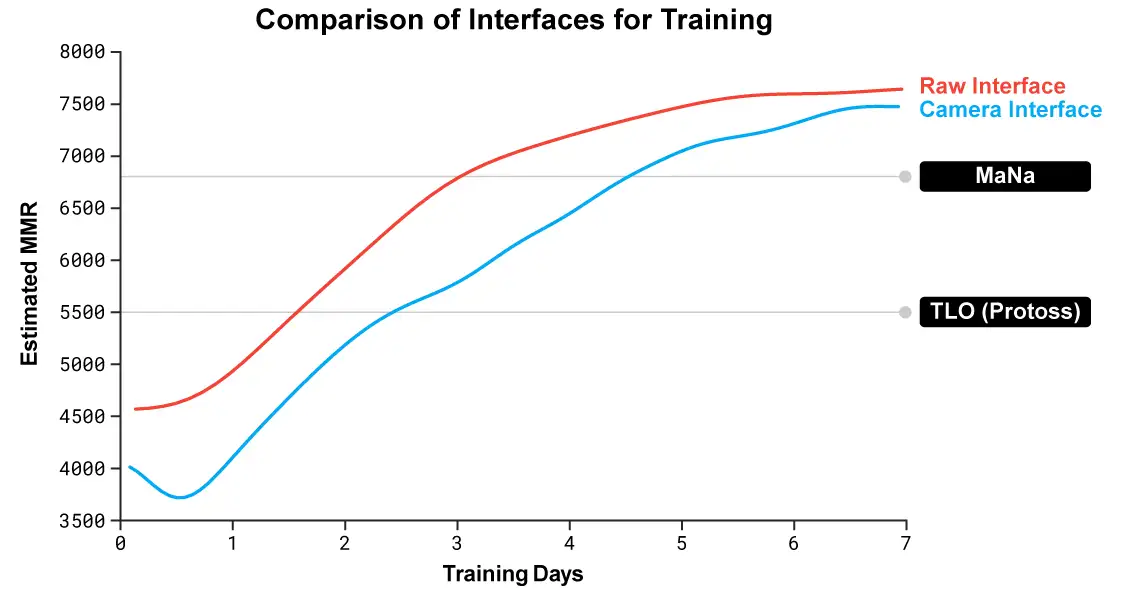
Another NN trained with camera-based interface lost the follow-up game against MaNa.

Partial observability: only see information in camera view, “saccade” actions
Imperfect information: only see opponent unit within range of own units
Large action space: simutaneous control of hundreds of units
Strategy cycles: counterstrategies discovered by pro players over 20 years

Relational inductive biases

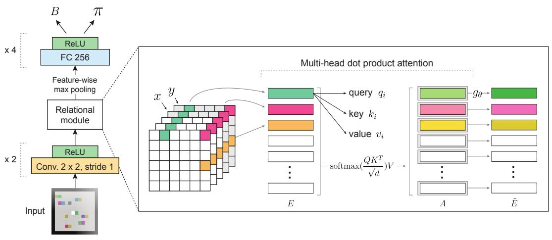
Vinicius et. al(2019)^[2] augmented model-free DRL with a mechanism for relational reasoning over structured representations via self-attention mechanisms, improving performance, learning efficiency, generalization and interpretability.

It incorporates relational inductive baises for entity- and relation- centric state representations, and iterated reasoning into the RL agent based on a distributed advantage actor-critic (A2C).

The agent receives the raw visual input pixels as the input, employing the front-end of CNNs to compute the entity embeddings, without depending on any priori knowledge, similar to Visual QA, video understanding tasks.

Embedded state representation

The agent creates an embedded state representation $S$ from its input observation, which is a spatial feature map returned by a CNN.

Relational module

Feature-to-entity transformation: the relational module reshapes the feature map $S$ (with shape $m \times n \times f$) to entity vectors $E$ (with shape $N \times f$, where $N=m \cdot n$). Each row of $E$, denoted as $\mathbf{e}_i$ , consists of a feature vector $\pmb{s}_{x,y}$ at a particular $x$,$y$ location in each feature map. This allows for non-local computation between entities, unconstrained by their coordinates in the spatial feature map.
Self-attention mechanism: apply multi-head dot-product attention(MHDPA) compute the pairwise interactions between each entity and all others (include itself). $A = \text{softmax}(d^{-1/2}QK^T)V$ where $d$ is the dimensionality of the query and key vectors.
Finally pass them to a multi-layer perceptron (MLP), with a residual connection. $\tilde{\pmb{e}}_i = g_\theta (\pmb{a}_i^{h=1:H})$

Output module

$\tilde{E}$ with the shape $N \times f$, is reduced to an $f$-dimensional vector by max-pooling over the entity dimension, followed by an MLP to output $(c+1)$-dimensional vector. The vector contains $c$-dimensional vector of $\pi$’s logits where $c$ is the # of discrete actions, plus a scalar baseline value estimate $B$.

Auto-regressive policy head

Vinyals et. al (2017)^[3] represented the policy with the auto-regressive manner, i.e. predict each action conditioned on previous actions:

$\pi_\theta(a \vert s) = \prod_{l=0}^L \pi_\theta (a^l \vert a^{<l}, s)$

The auto-regressive policy transforms the problem of choosing a full action $a$ to a sequence of decisions for each argument $a^l$.

Pointer Networks

It can be inferred that the Pointer Net is used to output the action for each unit, since the StarCraft involves many units in concert and the # of units changes over time. ^[6]

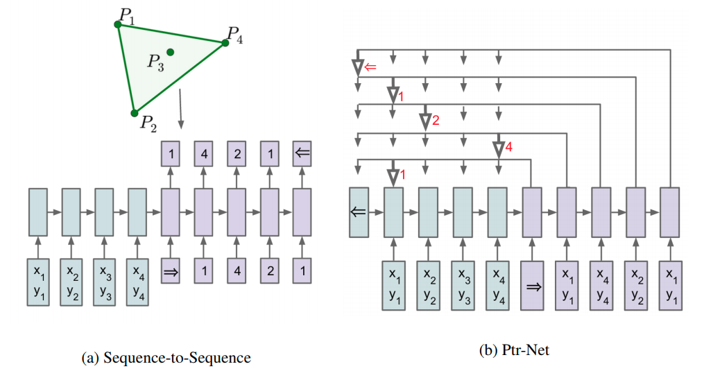
Pointer Net is employed to handle the variablity of the output length:

Applies the attention mechanism:
$u_j^i = v^T \tanh (W_1 e_j + W_2 d_i) \quad j \in (1,\cdots,n)$ $p(C_i \vert C_1, \cdots, C_{i-1}, \mathcal{P}) = \text{softmax}(u^i)$
where softmax normalizes the vector $u^i$ (of length $n$) to be an output distribution over the dictionary of inputs. And $v$, $W_1$ , $W_2$ are learnable parameters of the output model.

Here, we do not blend the encoder state $e_j$ to propagate extra information to the decoder $d_i$. Instead, we use $u_j^i$ as pointers to the input elements.

class Ptr(nn.Module):
	""" Pointer Nets """
    def __init__(self, h_size):
        super(Attn, self).__init__()
        self.h_size = h_size
        self.W1 = nn.Linear(h_size, h_size, bias=False)
        self.W2 = nn.Linear(h_size, h_size, bias=False)
        self.vt = nn.Linear(h_size, 1, bias=False)
        self.tanh = nn.Tanh()
        self.score = nn.Softmax(-1)

    def forward(self, dec, enc, m):
        attn = self.vt(self.tanh(self.W1(enc) + self.W2(dec))).squeeze(-1)
        logits = attn.masked_fill_(m, -float('inf'))
		return self.score(logits)

Ptr Nets can be seen as an application of content-based attention mechanisms.

Gated ResNet

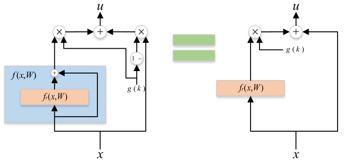
Gated Residual Network (Gated ResNet)^[20] adds a linear gating mechanism to shortcut connections using a scalar parameter to control each gate.

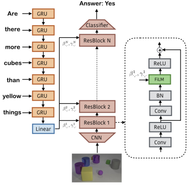
Let Residual layer $u = g(k) f(x, W) = f_r(x,W)+x$ , the gated Highway network is: $\begin{align} u &= g(k) f(x,W) + (1- g(k)) x \\ &= g(k) (\underbrace{f_r(x,W)+x}_\text{ResNet}) + (1-g(k))x \\ &= g(k)f_r(x,W) + x \end{align}$

FiLM

Feature-wise Liner Modulation (FiLM)^[21] applies the feature-wise affine transormation to the intermediate features of networks, based on some conditioning inputs.

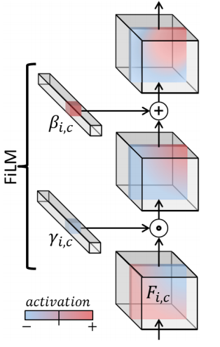
FiLM learns functions $f$ and $h$ which output $\gamma_{i,c}$ and $\beta_{i,c}$ as a function of input $\mathbf{x}_i$ :

$\begin{align} \gamma_{ic} & = f_c(\mathbf{x}_i) & \text{coefficient} \\ \beta_{i,c} &= h_c(\mathbf{x}_i) & \text{intercept} \\ \text{FiLM}(\mathbf{F}_{i,c} \vert y_{i,c}, \beta_{i,c}) &= \gamma_{i,c} \mathbf{F}_{i,c} + \beta_{i,c} & \text{FiLM generator} \end{align}$

where

$f$ and $h$ can be arbitary functions such as dense networks, sigmoid/tanh/exponential functions, etc.
Modulation of the target NN can be applied on the same input to that NN or some other inputs. For CNNs, $f$ and $h$ modulate the per-feature-map distribution of activations based on $\mathbf{x}_i$ .

FiLM-ed network architecture:

Centralized value baseline

Centralized critic

Problems: Conventional independent actor-critic (IAC) independently trains each agent, but the lack of information sharing impedes to learn coordinated strategies that depend on interactions between multiple agents, or to estimate the contribution of single agent’s action to the global rewards.
Solution: use a centralized critic that conditions on the true global state $s$, or the joint action-observation histories $\tau$ otherwise. (See the figure below)

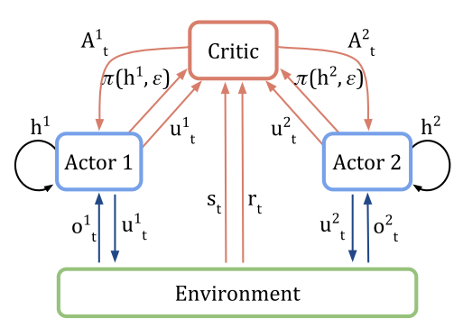
The critic (red parts in the figure) is used only during learning and only the actor is needed during execution.

Counterfactual baseline

Problems: A naive way is to follow the gradient based on the TD error: $g = \nabla_{\theta^\pi} \log \pi (\mu \vert \tau_t^a) (r+ \gamma V(s_{t+1})- V(s_t))$ It fails to address the key credit assignment problem since the TD error only considers global rewards, the gradient from each actor does not explicitly considered based on their respective contribution.
Solution: counterfactual baseline.
It is inspired by difference reward by computing the change of global reward when the action $a$ of an individual agent is replaced by a default action $c^a$: $D^a = r(s,\pmb{u}) - r(s, (\pmb{u}^{-a}, c^a))$

But difference baseline requires 1) the access to a simulator $r(s, (\pmb{u}^{-a}, c^a))$ and 2) a use-specific default action $c^a$.

counterfactual baseline. Compute the agent $a$ we can compute the advantage function that compares the $Q$-value for the current action $\mu^a$ to a counterfactual baseline that marginalize out $\mu^a$, while keeping the other agents’ actions $\mu^{-a}$ fixed: $A^a(s, \mu) = Q(s, \mu) - \sum_{\mu^{'a}} \pi^a(\mu^{'a} \vert \tau^a) Q(s, (\mu^{-a}, \mu^{'a}))$ where $A^a(s,\mu^a)$ measures the difference when only $a$’s action changes, learn directly from agents’ experiences rather than on extra simulations, a reward model or a use-designed default action.^[5]

Critic representation

The output dimension of networks would be equal to $|U|^n$, where $n$ is the # of agents. COMA uses critic representation in which it also takes the action of other agents $u_t^{-a}$ as part of the input, and output a $Q$-value for each of agent $a$’s action, with the # of output nodes $|U|$. (see Fig.(c) below)

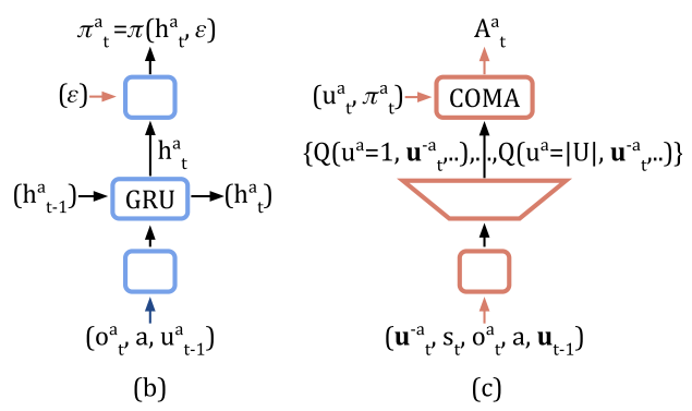
Fig. (b) and (c) are the architectures of the actor and critic.

Self-Imitation Learning

Self-Imitation Learning (SIL)^[8] learns to imitate the agent’s own past good experiences in the actor-critic framework. It stores experiences with cumulative rewards in a replay buffer: ${\mathcal{D}=\{ (s_t, a_t, R_t) \}}$ , where $s_t$ , $a_t$ are a state and an action at time-step $t$, and $R_t = \sum_{k=t}^\infty y^{k-t} r_k$ is the discounted sum of rewards with a discount factor $\gamma$, learns to imitate state-action pairs in the replay buffer only when the return in the past episode is greater than the agent’s value estimate.

Off-policy actor-critic loss

$\begin{align*} \mathcal{L}^\text{sil} &= \mathbb{E}_{s,a,R \in \mathcal{D}} [ \mathcal{L}^\text{sil}_\text{policy} + \beta^\text{sil} \mathcal{L}_\text{value}^\text{sil}] \\ \mathcal{L}_\text{policy}^\text{sil} &= -\log \pi_\theta (a \vert s) \max(R-V_\theta(s), 0) \\ \mathcal{L}_\text{value}^\text{sil} &= \frac{1}{2} || \max(R-V_\theta(s), 0) ||^2 \end{align*}$

where $\pi_\theta$ , $V_\theta(s)$ are the policy (i.e. actor) and the value function, $\beta^\text{sil} \in \mathbb{R}^+$ is a hyperparameter for the value loss.

The $\mathcal{L}_\text{policy}^\text{sil}$ can be interpreted as cross entropy loss with sample weights proportional to the gap between the return and the agent’s value estimate $(R-V_\theta)$ :

If the past return is greater than the agent’s value estimate, i.e. $R>V_\theta$ , the agent learns to choose the action chosen in the poast in the given state.
Otherwise ( $R < V_\theta$ ), such a state-action pair is not used to update due to the $\max$ op.
This encourages the agent to imitate its own decisions in the past only when such decisions resulted in larger returns than expected. $\mathcal{L}_\text{value}^\text{sil}$ updates the value estimate towards the off-policy return $R$.

Prioritized experience replay:

Sample transitions from the replay buffer using the clipped advantage $\max(R-V_\theta(s),0)$ as priority, i.e. sampling probablity is prop. to $\max(R-V_\theta(s),0)$ .

Advantage Actor-Critic with SIL (A2C + SIL)

A2C + SIL objective:

$\begin{align*} \mathcal{L}^\text{a2c} &= \mathbb{E}_{s,a\sim \pi_\theta} [\mathcal{L}_\text{policy}^\text{a2c} + \beta^\text{a2c} \mathcal{L}_\text{value}^\text{a2c}] \\ \mathcal{L}_\text{policy}^\text{a2c} &= - \log \pi_\theta (a_t \vert s_t) (V_t^n - V_\theta(s_t)) - \alpha \mathcal{H}_t^{\pi_\theta}\\ \mathcal{L}_\text{value}^\text{a2c} &= \frac{1}{2} ||V_\theta(s_t) - V_t^n||^2 \end{align*}$

SIL algorithms

Initialize parameter $\theta$
Initialize replay buffer $\mathcal{D} \leftarrow \emptyset$
Initialize episode buffer $\mathcal{E} \leftarrow \emptyset$
For each iteration do:
1. ## Collect on-policy samples
2. for each step do:
  1. execute an action $s_t, a_t, r_{t+1} \sim \pi_\theta(a_t \vert s_t)$
  2. store transition $\mathcal{E} \leftarrow \mathcal{E} \cup { (s_t, a_t, r_t) }$
3. if $s_{t+1}$ == TERMINAL:
  1. ## Update replay buffer
  2. compute returns $R_t = \sum_k^\infty \gamma^{k-t} r_k$ for all $t$ in $\mathcal{E}$
  3. $\mathcal{D} \leftarrow \mathcal{D} \cup { (s_t,a_t,R_t) }$ for all $t$ in $\mathcal{E}$
  4. clear episode buffer $\mathcal{E} \leftarrow \emptyset$
4. ## perform actor-critic using on-policy samples
5. $\theta \leftarrow \theta - \eta \nabla_\theta \mathcal{L}^\text{a2c}$
6. *## Perform self-imitation learning
7. for m = 1 to $M$:
  1. Sample a mini-batch ${ (s,a,R) }$ from $\mathcal{D}$
  2. $\theta \leftarrow theta - \eta \nabla_\theta \mathcal{L}^\text{sil}$

Policy distillation

Policy distillation is iused to train a new network that performs at the expert level while being dramatically smaller and more efficient ^[9]. Andrei et. al(2016) demonstrated that the multi-task distilled agent outperforms the single-task teachers as well as a jointly-trained DQN agent in the Atari domain.

Distillation

Distillation is proposed for supervised model compression, by creating a single network from an ensemble model. Model compression trains a student network using the output of a teacher network, compressing a large ensemble model into a single shallow network.

Single-game policy distillation

Distillation is to transfer knowledge frm a teacher model $T$ to a student model $S$.

The distillation targets from a classification targets from a classification network are typically obtained by passing the weighted sum of the last network layer through a softmax function.
In order to transfer more knowledge of the network, the teacher outputs can be softened by passing the network output through a relaxed (higher temperature) softmax than one that was used for training: $\text{softmax}(\frac{q^T}{\tau})$ , where $q^T$ is the vector of $Q$-values of $T$.

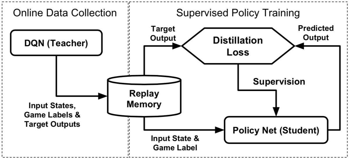
When transferring $Q$-value rather than a classifier, the scale of the $Q$-values may be hard to learn since it is not bounded and can be quite unstable. Training $S$ to predict only the single best action from $T$ is problematic, since multiple actions may have similar $Q$-values.

Consider policy distillation from $T$ to $S$, hwere the teacher $T$ generates a dataset $\mathcal{D}^T = \{ (s_i, q_i) \}_{i=0}^N$ , where each sample consists of a short observation sequence $s_i$ and unnormalized $Q$-value vector $q_i$ . Here is three approaches:

Only use the highest valued action from the teacher $a_\text{i, best} = \arg \max(q_i)$ . $T$ is trained with a negative log likelihood(NLL) to predict the same action: $L_\text{NLL}(\mathcal{D}^T, \theta_S) = - \sum_{i=1}^{|D|} \log P(a_i=a_\text{i, best} \vert x_i, theta_S)$
Train with mean-squared-error loss (MSE). It preserves the full set of action-values: $L_\text{MSE} (\mathcal{D}^T, \theta_S) = \sum_{i=1}^{|D|} || q_i^T - q_i^S ||_2^2$
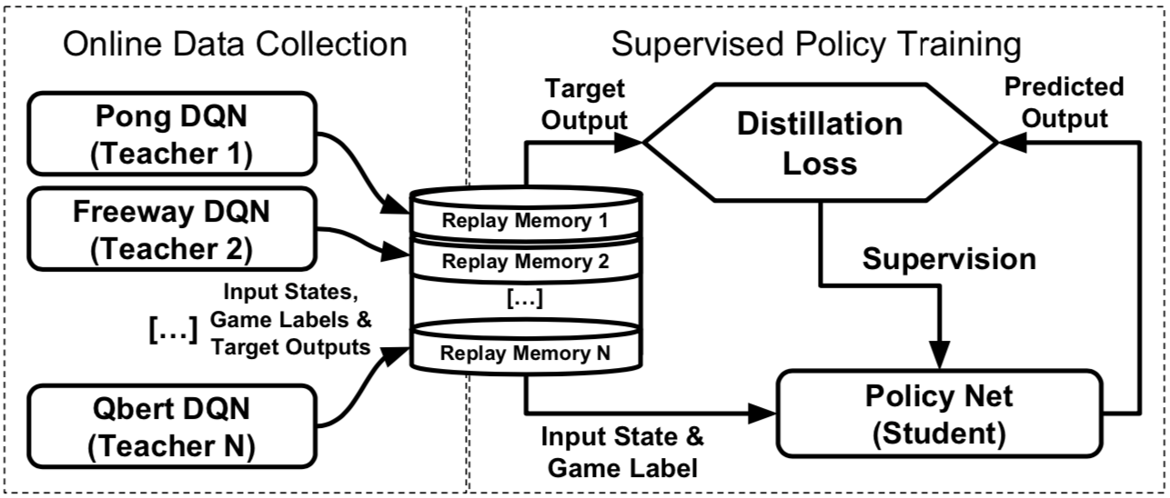
KL divergence with temperature $\tau$: $\begin{align} L_\text{KL} (\mathcal{D}^T, \theta_S) &= \text{KL} (\text{softmax}(\frac{q_i^T}{\tau}) || \text{softmax} (q_i^S) ) \\ &= \sum_{i=1}^{|D|} \text{softmax}(\frac{q_i^T}{\tau}) \ln \frac{\text{softmax}(\frac{q_i^T}{\tau})}{\text{softmax}(q_i^S)} \end{align}$

Multi-task policy distillation

Multi-task policy distillation uses $n$ DQN single-game experts, each trained separatedly, providing inputs and targets for $S$. The data is stored in separate memory buffers. The distillation agent $S$ learns from the $n$ data stores sequentially, and different tasks have different output layer(i.e. controller layer). The KL and NLL loss functions are used for multi-task distillation.

IMPALA

Importance Weighted Actor-Learning Architecture (IMPALA) can scale to thousands of machines without reducing data efficiency or resouce utilization. IMPALA achieves exceptionally high data throughput rates of 250,000 frames per second, over 30 times faster than single-machine A3C.^[10]

IMPALA archtecture

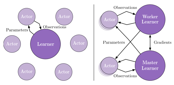
IMPALA applies an actor-critic setup to laern a policy $\pi$ and a baseline function $V^\pi$. Each actor updates its own local policy $\mu$ (i.e. behavior policy) to the latest learner policy $\pi$ (i.e. target policy), and runs $n$ steps in the environment. Afterwards, store the trajectory of states, actions, rewards, $\{(x_i,a_i,r_i) \}_{i=1}^n$ and policy distributions $\mu(a_t \vert x_t)$ as well as the initial LSTM state to a queue(as in left Fig.). This could lead to the policy-lag between actors and the learner. V-trace is proposed to correct the lag to get high data throughput while keeping data efficiency.

Also, IMPALA can employ synchronized parameter update (right fig.).^[10]

V-trace

V-trace target

Consider the trajectory $(x_t, a_t, r_t)_{t=s}^{t=s+n}$ generated by the actor following the some policy $\mu$, define $n$-step V-trace target for $V(s_s)$ , the value approximation at state $x_s$ :

$\begin{align*} v_s &\triangleq V(x_s) + \sum_{t=s}^{s+n-1} \gamma^{t-s}(\prod_{i=s}^{t-1}c_i) \pmb{\delta_t V} & \text{value approximation}\\ \pmb{\delta_t V} &\triangleq \rho_t (r_t + \gamma V(x_{t+1}) - V(x_t)) & \text{temporal difference for }V \\ \end{align*}$

where $\rho_t \triangleq \min(\bar{\rho}, \frac{\pi(a_t \vert x_t)}{\mu(a_t \vert x_t)})$ and $c_i \triangleq \min(\bar{c}, \frac{\pi(a_i \vert x_i)}{\mu(a_i \vert x_i)})$ are truncated improtance sampling(IS) weights.

The truncated IS weight $c_i$ define the fixed point of this update rule.
The weights $c_i$ are similar to the “trace cutting” coefficients in Retrace. The product $c_s \cdots c_{t-1}$ measures the temporal difference $\delta_t V$ observed at time $t$ impacts the value function update at previous time $s$.

V-trace actor-critic algorithms

At training time $s$, the value prameters $\theta$ are updated by gradient descent on $l2$ loss to the target $v_s$ , in the direction of: $(v_s - V_\theta(x_s)) \nabla_\theta V_\theta(x_s)$
update the policy params: $\rho_s \nabla_\omega \log \pi_\omega (a_s \vert x_s) (r_s + \gamma v_{s+1} - V-\theta(x_s))$
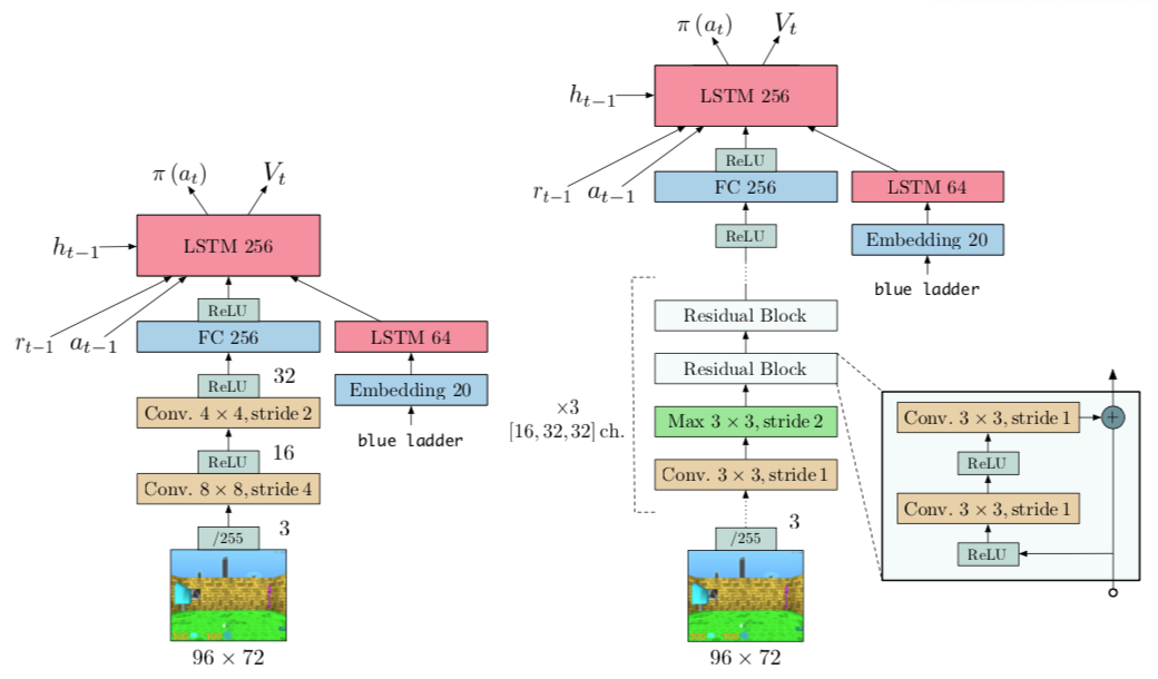
To prevent premature convergence, add an entropy term, along the direction: $- \nabla_\omega \sum_a \pi_\omega(a \vert x_s) \log \pi_\omega (a \vert x_s)$

Model

Left: small, 2 Conv layers, 1.2 million parameters;
Right: large, 15 Conv layers, 1.6 million parameters.

Population-based training(PBT)

Two common tracks of hyperparameter tuning:

parallel search:
- grid search
- random search
sequential optimization: requires multiple sequential training runs.
- Bayesian optimization

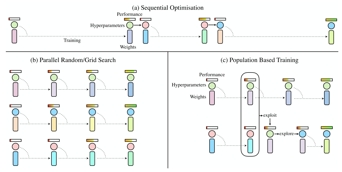
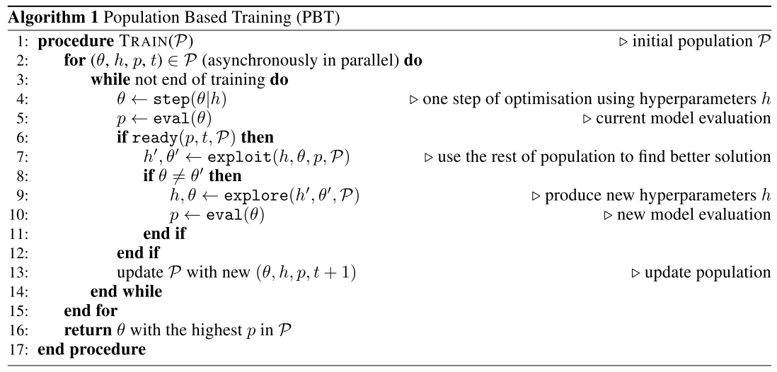
PBT starts like parallel search, randomly sampling hyperparameters and weight initializations. However, each training run asynchronously evaluates its performance periodically. If a model in the population is under-performing, it will exploit the rest of the polulation by replacing itself with a better performing model, and it will explore new hyperparameters by modifying a better model’s hyperparameters before training is continued.^[13]

PBT algorithms

Population-based Training(PBT) can be used to optimize neural networks for RL, supervised learning, GAN. PBT offers a way to optimize both the parameters $\theta$ and the hyperparameters $h$ jointly on the actual metric $\mathcal{Q}$ that we care about.

Training $N$ models $\{ \theta^i \}_{i=1}^N$ forming a population $\mathcal{P}$ which are optimized with different hyperparameters $\{ \mathbf{h}^i \}_{i=1}^N$ . Then use the collection of partial solutions in the population to perform meta-optimization, where the hyperparameters $h$ and weights $\theta$ are additionally adapted w.r.t the entire population. For each worker (member) in the population, we apply two functions independently:

expoit: decide whether the worker abandon the current solutions and copy a better one.
explore: propose new ones to better explore the solution space.

Each worker of the population is trained in paraleel, with iterative calls of the repeated cycle of local iterative training (with step) and exploitation and exploration with the rest of the population (with exploit and explore) until convergence of the model.

step: a step of gradient descent
eval: mean episodic return or validation set performance of the metric to optimize
exploit: select another member of the population to copy the weights and hyperparameters from
explore: create new hyperparameters for the next steps of gradient based learning by either perturbing the copied hyperparameters or resampling hyperparameters from the original defined prior distribution.

PBT is asynchronous and does not require a centralized process to orchestrate the training of the members of the population. “PBT is an online evolutionary process that adapts internal rewards and hyperparameters and performs model selection by replacing underperforming agents with mutated version of better agents”.^[14]

Silimar to genetic algorithms: local optimization by SGD -> periodic model selection -> hyperparameter refinement

PBT for RL

Hyperparameters: learning rate, entropy cost, unroll length for LSTM,…
Step: each iteration does a step of gradient descent with RMSProp on the model weights
Eval: evaluate the model with the last 10 episodic rewards during training
Ready: 1e6 ~ 1e7 agent steps finished

Exploit

T-selection: uniformly sample another agent in the population, and compare the last 10 episodic rewards using Welch’s t-test. If the sampled agent has a higher mean episodic reward and satisfies the t-test, the weights and hyperparameters are copied to replace the current agent.
Truncation selection: rank all agents in the population by episodic reward. Replace the bottom 20% agents with unformly sampled agent from the top 20% of the population, by copying the weights and hyperparameters.

Explore the hyperparameter space:

Perturb: randomly perturb each hyperparameter by a factor of 0.8 or 1.2 ($\pm 20\%$)
Resample: each hyperparameter is resampled from the original prior distribution defined with some probability.

For The Win (FTW)

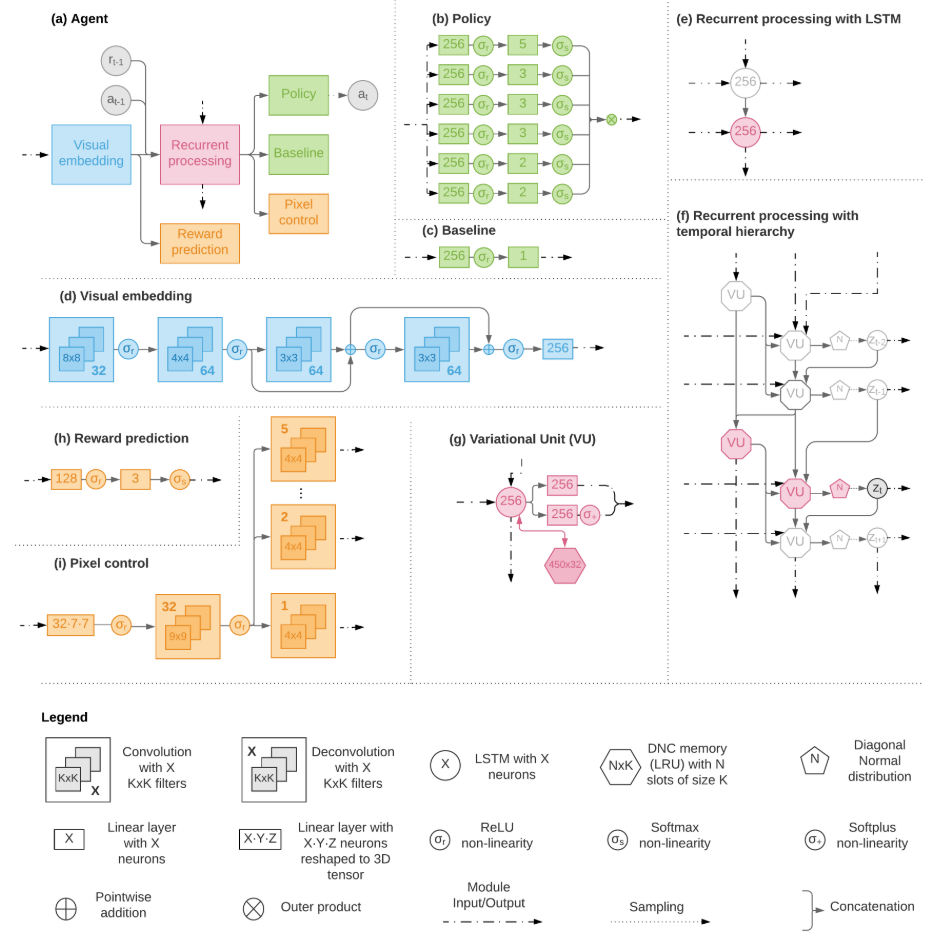
For The Win (FTW) network architecture:

Use a hirarchical RNN consisting of two RNNs, operating on two different timescales. The fast timescale RNN generates the hidden state $h_t^q$ at each time step $t$, while the slow timescale RNN produces the hidden state $h_t^p = h^p_{\tau \lfloor \frac{t}{\tau} \rfloor }$ every $\tau$ time steps.
The observation is encoded with CNNs.

PBT:

Optimize the hyperparameter $\phi$ of learning rate, slow LSTM time scale $\tau$, the weight of $D_\text{KL}$ term, entropy cost
In FTW, for each agent $i$ periodically sampled any agent $j$ and estimated the win probability of a team $i$ versus a team $j$. If the probabilty to win is less than 70%, the losing agent was replaced by the winner.
The exploration is perturbing the inherited value by $\pm 20\%$ with a probability of $5\%$, except that they uniformly sample the slow LSTM time scale $\tau$ from the integer range $[5,20)$.

Evolutionary computation

Lamarckian Evolution

PBT is a memetric algorithm that uses Lamarckian evolution (LE):

Innner loop: NNs are trained with backpropagation for individual solutions
Outer loop: evolution is run as the optimization algorithm, where NNs are picked with selection methods, with the winner’s parameters overwriting the loser’s.^[16]

Co-evolution

Competitive co-evolutionary algorithms(CCEAs) can be seen as a superset of self-play, it keep and evluate against an entire population of solutions, rather than keeping only one solution.

Quality diversity

Quality diversity (QD) algorithms explicitly optimize for a single objective(quality), but also searches for a large variety of solution types, via behaviour descriptors (i.e, solution phenotypes), to encourage greater diversity in the population.^[16]

For attribution in academic contexts, please cite this work as:

@misc{chai2019Decipher-AlphaStar-on-StarCraft-II,
  author = {Chai, Yekun},
  title = {{Deciphering AlphaStar on StarCraft II}},
  year = {2019},
  howpublished = {\url{https://cyk1337.github.io/notes/2019/07/21/RL/DRL/Decipher-AlphaStar-on-StarCraft-II/}},
}

References

1.Vaswani, A., Shazeer, N., Parmar, N., Uszkoreit, J., Jones, L., Gomez, A. N., ... & Polosukhin, I. (2017). Attention is all you need. In Advances in neural information processing systems (pp. 5998-6008). ↩
2.Zambaldi, V., Raposo, D., Santoro, A., Bapst, V., Li, Y., Babuschkin, I., ... & Shanahan, M. (2018). Deep reinforcement learning with relational inductive biases. ICLR 2019 ↩
3.Vinyals, O., Ewalds, T., Bartunov, S., Georgiev, P., Vezhnevets, A. S., Yeo, M., ... & Quan, J. (2017). Starcraft II: A new challenge for reinforcement learning. arXiv preprint arXiv:1708.04782. ↩
4.Vinyals, O., Fortunato, M., & Jaitly, N. (2015). Pointer networks. In Advances in Neural Information Processing Systems (pp. 2692-2700). ↩
5.Foerster, J. N., Farquhar, G., Afouras, T., Nardelli, N., & Whiteson, S. (2018, April). Counterfactual multi-agent policy gradients. In Thirty-Second AAAI Conference on Artificial Intelligence. ↩
6.https://www.alexirpan.com/2019/02/22/alphastar-part2.html ↩
7.COMA slides 2017, University of Oxford ↩
8.Oh, J., Guo, Y., Singh, S., & Lee, H. (2018). Self-imitation learning. arXiv preprint arXiv:1806.05635. ↩
9.Rusu, A. A., Colmenarejo, S. G., Gulcehre, C., Desjardins, G., Kirkpatrick, J., Pascanu, R., ... & Hadsell, R. (2015). Policy distillation. arXiv preprint arXiv:1511.06295. ↩
10.Espeholt, L., Soyer, H., Munos, R., Simonyan, K., Mnih, V., Ward, T., ... & Legg, S. (2018). Impala: Scalable distributed deep-rl with importance weighted actor-learner architectures. arXiv preprint arXiv:1802.01561. ↩
11.https://deepmind.com/blog/impala-scalable-distributed-deeprl-dmlab-30/ ↩
12.https://deepmind.com/blog/population-based-training-neural-networks/ ↩
13.Jaderberg, M., Dalibard, V., Osindero, S., Czarnecki, W. M., Donahue, J., Razavi, A., ... & Fernando, C. (2017). Population based training of neural networks. arXiv preprint arXiv:1711.09846. ↩
14.Jaderberg, M., Czarnecki, W. M., Dunning, I., Marris, L., Lever, G., Castaneda, A. G., ... & Sonnerat, N. (2019). Human-level performance in 3D multiplayer games with population-based reinforcement learning. Science, 364(6443), 859-865. ↩
15.https://deepmind.com/blog/capture-the-flag-science/ ↩
16.Arulkumaran, K., Cully, A., & Togelius, J. (2019). Alphastar: An evolutionary computation perspective. arXiv preprint arXiv:1902.01724. ↩
17.DeepMind AlphaStar: Mastering the Real-Time Strategy Game StarCraft II ↩
18.Vinyals, O., Babuschkin, I., Czarnecki, W. M., Mathieu, M., Dudzik, A., Chung, J., ... & Oh, J. (2019). Grandmaster level in StarCraft II using multi-agent reinforcement learning. Nature, 1-5. ↩
19.AlphaStar Nature paper supplemental data ↩
20.Savarese, P.H. (2017). Learning Identity Mappings with Residual Gates. ICLR ↩
21.Perez, E., Strub, F., Vries, H.D., Dumoulin, V., & Courville, A.C. (2017). FiLM: Visual Reasoning with a General Conditioning Layer. AAAI. ↩