Policy Gradient: A Summary !

The mathematical foundations of policy gradient algorithms.

Policy Gradient preliminaries

Policy gradient estimates the gradients with the form:^[10]

$$\nabla_\theta J(\theta) = \mathbb{E} \left[ \sum_{t=0}^{\infty} \Psi_t \nabla_\theta \log \pi_\theta (a_t \vert s_t) \right]$$

where $\Psi_t$ may be the following forms:

$$\begin{align} (1) \quad & \sum_{t=0}^\infty r_t & \text{total reward of the trajectory} &\\ (2) \quad & \sum_{t'=t}^\infty r_{t'} & \text{reward following action } a_t &\\ (3) \quad & \sum_{t'=t}^\infty r_{t'} - b(s_t) & \text{baselined version of (2)} &\\ (4) \quad & Q^\pi (s_t, a_t) & \text{state-action value function} &\\ (5) \quad & A^\pi(s_t, a_t) & \text{advantage function} &\\ (6) \quad & r_t+V^\pi(s_{t+1}) - V^{\pi}(s_t) & \text{TD residual} &\\ \end{align}$$

where (6) yields the lowest possible variance:

$$V^\pi (s_t) := \mathbb{E}_{s_{t+1:\infty}, \pmb{a_{t:\infty}} } \left[ \sum_{l=0}^\infty \gamma^l r_{t+l} \right]$$ $$Q^\pi (s_t, a_t) := \mathbb{E}_{s_{t+1:\infty}, \pmb{a_{t+1:\infty}} } \left[ \sum_{l=0}^\infty \gamma^l r_{t+l} \right]$$

The advantage function

$$A^\pi(s_t, a_t) := Q^\pi(s_t, a_t) - V^\pi (s_t)$$

• Intuitional interpretation: a step in policy gradient direction should increase the probability of better-than-average actions and decrease the probability of worse-than-average actions. The advantage function measures whether or not the action is better or worse than the policy’s default behavior (expection).

Vanilla Policy Gradient

The goal of RL

Objective

$$\theta^* = \arg \max_\theta E_{\tau \sim p_\theta(\tau)} \big[ \sum_t r\mathbf{(s_t,a_t)} \big]$$

• Infinite horizon $$\theta^{*} = \arg \max_{\theta} E_{\mathbf{(s,a)} \sim p_\theta \mathbf{(s,a)}} [r \mathbf{(s,a)}]$$
• Finite horizon $$\theta^* = \arg\max_\theta \sum_{t=1}^T E_{ \mathbf{(s_t,a_t)} \sim p_\theta \mathbf{(s_t,a_t)} } \big[ r \mathbf{(s,a)} \big]$$

Evaluating the objective

$$\theta^* = \arg\max_\theta \underbrace{E_{\tau \sim p_{\theta}(\tau)} \big[ \sum_t r (\mathbf{s}_t,\mathbf{a}_t) \big]}_{J(\theta)}$$ $$J(\theta) = E_{\tau \sim p_{\theta}(\tau)} \big[ \sum_t r (\mathbf{s}_t,\mathbf{a}_t) \big] \approx \frac{1}{N} \underbrace{\sum_i \sum_t r(\mathbf{s}_{i,t}, \mathbf{a}_{i,t}) }_{i \rightarrow \text{sum over samples from } \pi_\theta}$$

Direct differentiation

$$J(\theta) =E_{\tau \sim \pi_{\theta}(\tau)} \big[ r(\tau) \big] = \int \pi_\theta (\tau) r(\tau) d \tau$$ $$r(\tau) = \sum_{t=1}^T r(\mathbf{s}_t, \mathbf{a}_t)$$ $$\begin{align} \nabla_\theta J(\theta) & = \int \nabla_\theta \pi_\theta (\tau) r(\tau) d \tau \\ &= \int \pi_\theta (\tau) \nabla_\theta \log \pi_\theta (\tau) r(\tau) d \tau \\&= E_{\tau \sim \pi_{\theta}(\tau)} \big[ \nabla_\theta \log \pi_\theta (\tau) r(\tau) \big] \end{align}$$

A convenient identity:

$$\pi_{\theta}(\tau) \nabla_\theta \log \pi_\theta (\tau) = \pi_\theta (\tau) \frac{\nabla_\theta \pi_\theta (\tau)}{\pi_\theta (\tau)} = \nabla_\theta \pi_\theta (\tau)$$

$$\begin{align} \log \pi_\theta(\tau) &= \log \pi_\theta(\mathbf{s}_1,\mathbf{a}_1, \cdots, \mathbf{s}_T,\mathbf{a}_T) \\&= \log \big[ p(\mathbf{s}_1) \prod_{t=1}^T \pi_\theta (\mathbf{a}_t \vert \mathbf{s}_t) p(\mathbf{s}_{t+1} \vert \mathbf{s}_t,\mathbf{a}_t ) \big ] \\ &= \underbrace{\log p(\mathbf{s}_1)}_\text{initial probability, derivative:0} + \underbrace{\sum_{t=1}^T \log \pi_\theta (\mathbf{a}_t \vert \mathbf{s}_t)}_\text{transition prob.} + \underbrace{\log p(\mathbf{s}_{t+1} \vert \mathbf{s}_t,\mathbf{a}_t )}_\text{emission prob., derivative:0} \end{align}$$

Overall,

$$\begin{align} \nabla_\theta J(\theta) &= E_{\tau \sim \pi_\theta(\tau)} [\nabla_\theta \log \pi_\theta(\tau) r(\tau)] \\&= E_{\tau \sim \pi_\theta(\tau)} \big[ \big( \sum_{t=1}^T \log \pi_\theta (\mathbf{a}_t \vert \mathbf{s}_t) \big ) \big( \sum_{t=1}^T r(\mathbf{s}_t, \mathbf{a}_t) \big) \big] \\& \approx \frac{1}{N} \sum_{i=1}^N \big( \sum_{t=1}^T \nabla_\theta \log \pi_\theta (\mathbf{a}_{i,t} \vert \mathbf{s}_{i,t}) \big) \big( \sum_{t=1}^T r(\mathbf{s}_{i,t} , \mathbf{a}_{i,t}) \big) \end{align}$$

• Comparison to Maximum likelihood: $$\nabla_\theta J_{ML}(\theta) \approx \frac{1}{N} \sum_{i=1}^N \big( \sum_{t=1}^T \nabla_\theta \log \pi_\theta (\mathbf{a}_{i,t} \vert \mathbf{s}_{i,t}) \big)$$

Drawbacks: variance

• Reducing variance

• Future does not affect the past
• Casuality: policy at time $t’$ cannot affect reard at time t when $t<t’$

$$\nabla_\theta J(\theta) \approx \frac{1}{N} \sum_{i=1}^N \sum_{t=1}^T \nabla_\theta \log \pi_\theta (\mathbf{a}_{i,t} \vert \mathbf{s}_{i,t}) \hat{Q}_{i,t}$$

where $\hat{Q}_{i,t}$ denotes the reward to go:

$$\hat{Q}_{i,t} = \sum_{t'=i}^T r(\mathbf{s}_{i,t'}, \mathbf{a}_{i,t'})$$

Baselines

$$\nabla_\theta J(\theta) \approx \frac{1}{N} \sum_{i=1}^N \nabla_\theta \log \pi_\theta (\tau) [r(\tau)-b]$$

where $b=\frac{1}{N} \sum_{i=1}^N r(\tau)$

proof:

• Substracting abseline is unbiased in expectation

• Average reward is not the best baseline, but it’s pretty good.

  $$E[\nabla_\theta \log \pi_\theta(\tau) b] = \int \pi_\theta (\tau) \nabla_\theta \log \pi_\theta (\tau) b d\tau = \int \nabla_\theta \pi_\theta (\tau)b d\tau = b \nabla_\theta \int \pi_\theta(\tau) d\tau =b\nabla_\theta 1 = 0$$

• Optimal baseline:

  $$\text{var}[x] = E[x^2] - E[x]^2$$ $$\nabla_\theta J(\theta) = E_{\tau \sim \pi_\theta(\tau)} [\nabla_\theta \log \pi_\theta(\tau)(r(\tau)-b)]$$

$$\text{var} = E_{\tau \sim \pi_\theta(\tau)} [(\nabla_\theta \log \pi_\theta (\tau) (r(\tau)-b))^2] - E_{\tau \sim \pi_\theta(\tau)} [\underbrace{\nabla_\theta \log \pi_\theta (\tau) (r(\tau)-b)}_{\text{this is just unbiased baseline in expectation}}]^2$$

Hence,

$$\frac{d \text{var}}{db} = \frac{d}{db} E[g(\tau)^2(r(\tau)-b)^2] = \frac{d}{db} \big( E[g(\tau)^2 r(\tau)^2] - 2E[g(\tau)^2 r(\tau) b] + b^2 E[g(\tau)^2] \big) \\= -2 E[g(\tau)^2 r(\tau)] + 2b E[g(\tau)^2] = 0$$

We get:

$$b = \frac{E[g(\tau)^2 r(\tau)]}{E[g(\tau)^2]}$$

This is just the expected reward, weighted by gradient magnitudes.

Deriving the simplest policy gradient (Spinning Up)

Consider the case of a stochastic, parameterized policy, $\pi_{\theta}$. We maximize the expected return

$$J(\theta) = \underset{\tau \sim \pi_\theta}{R(\tau)}$$

Optimize the policy by gradient descent:

$$\theta_{k+1} = \theta_k + \alpha \underbrace{\nabla_\theta J(\pi_{\theta})\vert_{\theta_k}}_\text{policy gradient}$$

Step by step:

1. Probability of a Trajectory. The probability of a trajectory $\tau = (s_0, a_0, \cdots, s_{T+1})$ given that actions come from $\pi_\theta$ is:

   $$P(\tau \vert \theta) = \rho_0(s_0) \prod_{t=0}^T P(s_{t+1} \vert s_t, a_t) \pi_\theta (a_t \vert s_t)$$

2. The log-derivative trick.

   $$\nabla_\theta P(\tau \vert \theta) = P(\tau \vert \theta) \nabla_\theta \text{log} P(\tau \vert \theta)$$

3. Log-probability of a trajectory:

   $$\text{log} P(\tau \vert \theta) = \text{log} \rho_0 (s_0) + \sum_{t=0}^T \big( \text{log}P(s_{t+1} \vert s_t,a_t) + \text{log} \pi_\theta (a_t \vert s_t) \big)$$
4. Gradients of environment functions
   The environment has no dependence on $\theta$, so gradients of $\rho_0(s_0)$, $P(s_{t+1} \vert s_t, a_t)$ and $R(\tau)$ are zero.
5. Grad-log-prob of a trajectory.
   The gradient of the log-prob of a trajectory is thus

Overall:

$$\begin{align} \nabla_\theta J(\pi_\theta) & = \underset{\tau \sim \pi_\theta}{E} [R(\tau)] \\ & = \nabla_\theta \int_\tau P(\tau \vert \theta) R(\tau) & \text{expand expectation}\\ & = \int_\tau \nabla_\theta P(\tau \vert \theta) R(\tau) & \text{bring gradient under integral}\\ & = \int_\tau P(\tau \vert \theta) \nabla_\theta \log P(\tau \vert \theta) R(\tau) & \text{log-derivative trick}\\ & = \underset{\tau \sim \pi_\theta}{E} \big[ \nabla_\theta \log P(\tau \vert \theta) R(\tau) \big] & \text{return to expectation form} \end{align} \\ \therefore \nabla_\theta J(\pi_\theta) = \underset{\tau \sim \pi_\theta}{E} \big[ \sum_{t=0}^T \nabla_\theta \log P(\tau \vert \theta) R(\tau) \big]$$

We can estimate the expectation with a sample mean. If we collect a set of trajectories $\mathcal{D} = \{ \tau_i \}_{i=1,\cdots,N}$ where each trajectory is obtained by letting the agent act in the environment using the policy $\pi_\theta$, the policy gradient can be estimated as:

$$\hat{g} = \frac{1}{|D|} \sum_{\tau \in \mathcal{D}} \sum_{t=0}^T \nabla_\theta \text{log} \pi_\theta (a_t \vert s_t) R(\tau)$$

where $|\mathcal{D}|$ is the # of trajectories in $\mathcal{D}$

REINFORCE

REINFORCE(Monte-Carlo policy gradient) is a Monte-Carlo algorithm using the complete return from the time $t$, which includes future rewards up until the end of episode. ^[3]

$$\begin{align} \nabla J(\theta) & = \mathbb{E}_\pi \left[ \sum_a \pi(a \vert S_t, \theta) q_\pi (S_t, a) \frac{\nabla \pi(a \vert S_t, \theta)}{\pi(a \vert S_t, \theta)} \right] \\ & = \mathbb{E} \left[ q_\pi(S_t, A_t) \frac{\nabla \pi(A_t \vert S_t,\theta)}{\pi(A_t \vert S_t, \theta)} \right] \\ & = \mathbb{E} \left[ G_t \underbrace{\frac{\nabla \pi(A_t \vert S_t,\theta)}{\pi(A_t \vert S_t, \theta)}}_{\text{eligibility vector:} \\ \nabla \ln \pi(A_t \vert S_t,\theta)} \right] \end{align}$$

• Intuition: the update increases the paramer vector in this distribution proportional to the return, and inversely proportional to the action probability.

REINFORCE algorithm:

1. Initialize policy parameter $\theta$ at random;
2. For each episode:
   1. Generate an episode $S_0, A_0, R_1, \cdots, S_{T-1}, A_{T-1}, R_T$, following $\pi(\cdot \vert \cdot, \theta)$
   2. Loop for each step of the episode $t=0,1,\cdots, T-1$:
      1. $ G \leftarrow \sum_{k=t+1}^T \gamma^{k-t-1} R_k $
      2. $\theta \leftarrow \theta + \alpha \gamma^t G \nabla \ln \pi (A_t \vert S-t, \theta)$

• Drawbacks: REINFORCE has a high variance and thus produces slow learning.

REINFORCE with Baseline

A variant of REINFORCE is to substract a baseline value from the return $G_t$ to reduce the variance of policy gradient while keeping the bias unchanged.^[3]

$$\theta_{t+1} = \theta_t + \alpha \left( G_t - \pmb{b(S_t)}\right) \nabla \ln \pi(A_t \vert S_t, \theta_t)$$

Actor-Critic

Actor-Critic consists of two components

Actor-Critic algorithms:

1. Initialize policy parameter $\pmb{\theta} \in \mathbb{R}^{d’}$ and state-value weights $\pmb{w} \in \mathbb{R}^d$
2. For each episode:
   1. Initilize the first state of episode $ S \leftarrow 1$
   2. While $S$ != TERMINAL (for each time step):
      1. $A \sim \pi(\cdot \vert S,\theta) $
      2. Take action $A$, observe $S’$, $R$
      3. $\delta \leftarrow R + \gamma \hat{v}(S’,\pmb{w}) - \hat{v}(S,\pmb{w})$ (If $S’$ is terminal, then $\hat{v}(S’, \pmb{w})=0$)
      4. $\pmb{w} \leftarrow \pmb{w} + \alpha^{\pmb{w}} \delta \nabla \hat{v}(S,\pmb{w})$
      5. $\pmb{\theta} \leftarrow \pmb{\theta} + \alpha^{\theta} I \delta \nabla \ln \pi(A \vert S,\theta)$
      6. $I \leftarrow \gamma I$
      7. $S \leftarrow S’$

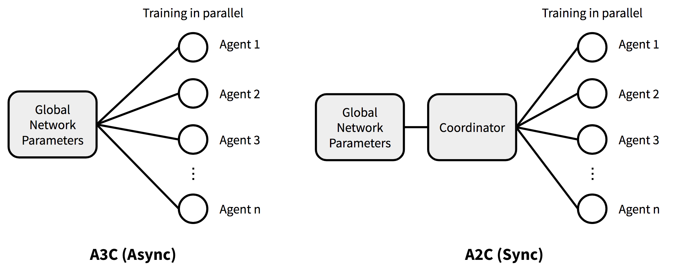
Asynchronous Advantage Actor-Critic(A3C)

Mnih et.al(2016) ^[1] proposed an asynchronous gradient descent for optimization of deep neural networks, showing that parallel actor-learners have a stabilizing effect on training, greatly reducing the training time with a single multi-core CPU instead of GPU.

• Instead of experience replay, they asynchronously execute multiple agents in parallel on multiple instances of the environment. This parallelism also decorrelates the agents’ data into a more stationary process, since at any given time-step the parallel agents will be experiencing a variety of different states.
• Apply different exploration policies in each actor-learner to maximize the diversity. By running different exploration policies in different threads, the overall updates of parameters are likely to be less correlated in time than a single agent applying online updates.
• The gradient accumulation in parallelism can be seen as a prarallized minibatch of stochastic gradient update, where the parameters update thread-by-thread in the direction of each thread independently.^[2]

A3C pseudocode for each actor-learner thread:

1. Assume global shared parameter vectors $\theta$ and $\theta_v$ and global shared counter $T=0$, thread-specified parameter vectors $\theta’$ and $\theta’_v$
2. Initialize the thread step count $t \leftarrow 1$
3. While $T<=T_{max}$:
   1. Reset gradients: $d\theta \leftarrow 0$ and $d\theta_v \leftarrow 0$
   2. Synchronize thread-specific parameters $\theta’=\theta$ and $\theta’_v = \theta_v$
   3. $t_\text{start} = t$
   4. sample state $s_t$
   5. while ($s_t$ != TERMINAL and $t - t_\text{start} <= t_\text{max}$):
      1. Perform the action $a_t \sim \pi(a_t \vert s_t; \theta')$
      2. Receive reward $r_t$ and new state $s_{t+1}$;
      3. $t \leftarrow t+1$
      4. $T \leftarrow T+1$
   6. The return estimation: $$R = \begin{cases} 0 & \text{if } s_t \text{ is TERMINAL} \\ V_{w’}(s_t) & \text{otherwise}\end{cases}$$
   7. For $i \in \{ t-1, \cdots, t_\text{start} \}$ do
      1. $R \leftarrow \gamma R + R_i$; here $R$ is a MC measure of $G_i$
      2. Accumulate gradients w.r.t $\theta’$: $d\theta \leftarrow d\theta + \nabla_{\theta'} \log \pi(a_i \vert s_i;\theta') (R-V(s_i;\theta_v'))$
      3. Accumulate gradients w.r.t $d\theta_v \leftarrow d\theta_v + \frac{\partial (R-V(s_i;\theta_v'))^2}{\partial \theta_v'}$
   8. Perform asynchronous update of $\theta$ using $d\theta$ and of $\theta_v$ using $d\theta_v$

Advantage Actor-Critic (A2C)

Removing the first “A”(Asynchronous) from A3C, we get advantage actor-critic (A2C). A3C updates the global parameters independently, thus thread-specific agents updates the policy with different versions and aggregated updates could not be optimal.

A2C waits for each actor to finish its segment of experience before performing an update, averaging over all of the actors. In the next iteration, parallel actors starts from the same policy. A2C is more cost-effective than A3C when using single-GPU machines, and is faster than a CPU-only A3C implementation when using larger policies. ^[4]

Trust Region Policy Optimization (TRPO)

Trust Region Policy Optimization (TRPO) enforces a KL divergence constraint at every point in the state space.

TRPO minimizes a certain surrogate obejctive fuction guarateeing policy improvement with non-trivial step sizes, giving monotonic improvements with little tuning of hyperparameters at each update^[5].

• Let $\tilde{\pi}$ denote the expected return of another policy $\tilde{\pi}$ in terms of the advantage over the policy $\pi$
• $\rho_\pi$ denotes discounted visitation frequency: $\rho_\pi (s) = P(s_0=s) + \gamma P(s_1 = s) + \gamma^2 P(s_2=s)+ \cdot$.

$$\begin{align} \eta(\tilde{\pi}) &= \eta(\pi) + \mathbb{E}_{s_0,a_0,\cdots \sim \tilde{\pi}} \left[ \sum_{t=0}^\infty \gamma^t A_\pi (s_t, a_t) \right] & \\ & = \eta(\pi) + \sum_s \pmb{\rho_{\tilde{\pi}}}(s) \sum_{a} \tilde{\pi} (a \vert s) A_\pi (s,a) & \text{rewrite with sum over states} \\ L_\pi(\tilde{\pi})& \approx \eta(\pi) + \sum_s \pmb{\rho_{\pi}}(s) \sum_{a} \tilde{\pi} (a \vert s) A_\pi (s,a) & \text{replace } \rho_{\tilde{\pi}} \text{ with } \rho_{\pi} \text{ to approximate} \\ \end{align}$$

The aforementioned update does not give any guidance on the step size to update.

• Conservative policy iteration provides explicit lower bounds on the improvements of $\eta$.

Let $\pi_\text{old}$ denote the current policy and $\pi' = \arg \max_{\pi'} L_{\pi_\text{old}} (\pi')$, the new policy is:

$$\pi_\text{new}= (1-\alpha)\pi_\text{old} (a \vert s) + \alpha \pi'(a \vert s)$$

where the lower bound:

$$\begin{align} \eta(\pi_\text{new}) &\geq L_{\pi_\text{old}}(\pi_\text{new}) - \frac{2 \epsilon \gamma}{(1-\gamma)^2}\alpha^2 & \\ & \text{where } \epsilon = \max_s \vert \mathbb{E}_{a \sim \pi'(a \vert s)} [A_\pi (s,a)] \vert & \\ \end{align}$$

Replace $\alpha$ with the distance measure between $\pi$ and $\tilde{\pi}$, total vairation divergence: $D_\text{TV}=\frac{1}{2} \sum_i |p_i - q_i|$ for discrete distributions $p,q$.
Define $D_\text{TV}^{\max} = \max_{s,a} |A_\pi (s,a)|$

$$\begin{align} \eta(\pi_\text{new}) & \geq L_{\pi_\text{old}}(\pi_\text{new}) - \frac{4 \epsilon \gamma}{(1-\gamma)^2}\alpha^2 & \text{replace } \alpha \text{ with total variation divergence} \\ & \text{where } \epsilon =\max_{s,a} | A_\pi (s,a)| & \end{align}$$

Since $D_{TV} (p || q)^2 \leq D_{KL}(p || q)$, Let $D_{KL}^{\max} (\pi, \tilde{\pi}) = \max_s D_{KL}(\pi(\cdot \vert s) || \tilde{\pi}(\cdot \vert s))$, we get:

$$\begin{align} \eta(\pi) & \geq L_\pi (\tilde{\pi} - C D_{KL}^{\max}(\pi, \tilde{\pi})) & \text{replace } \alpha^2 \text{ with } D_{KL}^{\max} (\pi, \tilde{\pi}) \\ & \text{where } C=\frac{4 \epsilon \gamma}{(1-\gamma)^2} \end{align}$$

Let $M_i(\pi) = L_{\pi_i} (\pi) - C D_{KL}^{\max}(\pi_i, \pi)$, then:

$$\begin{align} \eta(\pi_{i+1}) \geq M_i (\pi_{i+1}) & \\ \eta(\pi_i) = M_i(\pi_i) &\\ \end{align}$$

Therefore,

$$\eta(\pi_{i+1}) - \eta(\pi_i) \geq M_i(\pi_{i+1}) - M (\pi_i)$$

This guarantees that the true objective $\eta$ is non-decreasing.

Afterwards, we improve the true objective $\eta$. Let $\theta_\text{old}$ represent $\pi_{\theta_\text{old}}$, and $\theta$ represent $\pi_\theta$.

$$\text{maximize}_{\theta} [ L_{\theta_\text{old}}(\theta) - C D_\text{KL}^{\max} (\theta_\text{old}, \theta)]$$

Thus, we use a constraint on the KL divergence beween the new policy and the old policy, i.e., a trust region constraint:

$$\begin{align} \text{maximize}_{\theta} L_{\theta_\text{old}}(\theta) & \\ s.t. D_\text{KL}^{\max} (\theta_\text{old}, \theta) \leq \delta & \end{align}$$

By heuristic approximation, we consider the average KL divergence to replace the $\max$ KL divergence:

$$\begin{align} & \text{maximize}_{\theta} L_{\theta_\text{old}}(\theta) \\ & s.t. \bar{D}_\text{KL}^{\rho_{\theta_\text{old}}} (\theta_\text{old}, \theta) \leq \delta \\ \end{align}$$

• Expand $L_{\theta_\text{old}}$: $$\text{maximize}_{\theta} \sum_s \rho_{\theta_\text{old}}(s) \sum_a \pi_\theta (a \vert s) A_{\theta_\text{old}}(s,a)$$
• Replace the sum over actions by an important sampling estimator: $$\sum_a \pi_\theta(a \vert s_n) A_{\theta_\text{old}} (s_n, a) = \mathbb{E}_{a \sim q} \left[ \frac{\pi_\theta(a \vert s_n)}{q(a \vert s_n)} A_{\theta_\text{old}}(s_n, a) \right]$$
• Replace $\sum_s \rho_{\theta_\text{old}}$ with expectation $\mathbb{E}_{s \sim \rho_{\theta_\text{old}}}[\cdots]$; replace the advantage values $A_{\theta_\text{old}}$ by the $Q$-values $Q_{\theta_\text{old}}$. Finally, we get $$\begin{align} \text{maximize}_\theta & \mathbb{E}_{s \sim \rho_{\theta_\text{old}}, a \sim q} \left[ \frac{\pi_\theta (a \vert s)}{q(a \vert s)} Q_{\theta_\text{old}}(s,a) \right] \\ s.t. & \mathbb{E}_{s \sim \rho_{\theta_\text{old}}} \left[ D_\text{KL} \left(\pi_{\theta_\text{old}}(\cdot \vert s) || \pi_\theta (\cdot \vert s) \right) \right] \leq \delta \end{align}$$

Proximal Policy Optimization (PPO)

• Problems: TRPO is relatively complicated, and is not compatible with architectures that include noise (e.g. dropout) or parameter sharing (between the policy and value function, or with auxiliary tasks).^[8]

• PPO with clipped surrogate objective performs better than that with KL penalty.

PPO-clip *

Clipped surrogate objective

• Let $r_t(\theta) = \frac{\pi_\theta (a_t \vert s_t)}{\pi_{\theta_\text{old}}(a_t \vert s_t)}$, so $r(\theta_\text{old})=1$. TRPO maimize a surrogate objective with conservative policy iteration (CPI). Without the constraint, maximization of $L^{\text{CPI}}$ would lead to excessively large policy update. $$\begin{align} L^{\text{CPI}}(\theta) & = \hat{\mathbb{E}}_t \left[ \frac{\pi_\theta (a_t \vert s_t)}{\pi_{\theta_\text{old}}(a_t \vert s_t)} \hat{A}_t \right] = \hat{\mathbb{E}}_t \left[ r_t(\theta) \hat{A}_t \right] \\ s.t. & \hat{\mathbb{E}}_t \left[ \text{KL} [\pi_{\theta_\text{old}} (\cdot \vert s_t), \pi_\theta (\cdot \vert s_t) ] \right] \leq \delta \end{align}$$
• PPO pernalize changes to the policy that move $r_t(\theta)$ away from 1: $$L^\text{clip}(\theta) = \hat{\mathbb{E}} \left[ \min \big( r_t(\theta)\hat{A}_t, \text{clip}(r_t(\theta), 1-\epsilon, 1+\epsilon) \hat{A}_t \big) \right]$$

where $\epsilon$ is a hyperparameter, say, $\epsilon=0.2$. The intuition is to take the minimum of the clipped and unclipped objective, thus the final objective is a lower bound (i.e. a pessimistic bound) on the unclipped objective.

PPO-penalty

Adaptive KL pernalty coefficient

• Variant: add a penalty on KL divergence
• With mini-batch SGD, optimize the KL-penalized objective: $$L^\text{KL-penalty} = \hat{\mathbb{E}} \left[ \frac{\pi_\theta (a_t \vert s_t)}{\pi_{\theta_\text{old}}} \hat{A}_t - \beta \text{KL} [ \pi_{\theta_\text{old}} (\cdot \vert s_t), \pi_\theta (\cdot \vert s_t) ] \right]$$
• Compute $d=\hat{E}_t [\text{KL} [ \pi_{\theta_\text{old}} (\cdot \vert s_t), \pi_\theta (\cdot \vert s_t) ] ]$
  • If $d < d_\text{target}/1.5, \beta \leftarrow \beta/2$
  • If $d > d_\text{target} \times 1.5, \beta \leftarrow \beta \times 2$

PPO algorithms

Finally, the objective function is augmented with an error term on the value estimation and an entropy term to encourage sufficient exploration.

$$\begin{align} L^\text{Clip + SE + Entropy}_t (\theta) = \mathbb{E} \left[ L^\text{clip}_t (\theta) - c_1 \underbrace{(V_\theta (s_t) - V_t^\text{target})^2}_\text{squared error loss} + c_2 \underbrace{\mathbb{H}(s_t, \pi_{\theta})}_\text{entropy term} \right] \end{align}$$

where $c_1$, $c_2$ are constant coefficients.

• Settings:
  • RNN
  • Adam
  • mini-batch SGD

PPO algorithms with Actor-Critic style:

1. for iteration=$1,2,,\cdots$:
   1. for actor=$1,2,,\cdots, N$:
      1. run policy $\pi_{\theta_\text{old}}$ in environment for $T$ timesteps;
      2. Compute advantage estimates $\hat{A}_1, \cdots, \hat{A}_T$;
   2. Optimize surrogate $L$ w.r.t $\theta$, with $K$ epochs and mini-batch size $M \leq NT$
   3. $\theta_\text{old} \leftarrow \theta$

Distributed PPO

Let $W$ denote # of workers; $D$ sets a threshold for the # of workers whose gredients must be available to update the parameters; $M$, $B$ is the # of sub-iterations with policy and baseline updates given a batch of datapoints.^[9]

The distributed PPO-penalty algorithms:

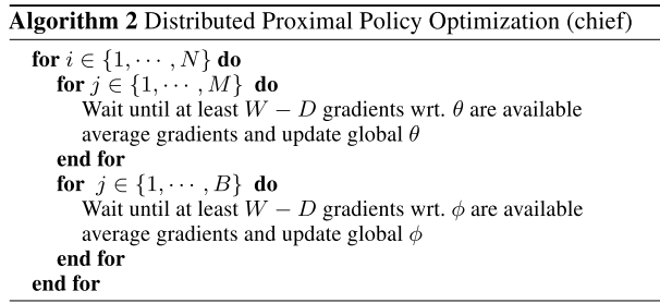
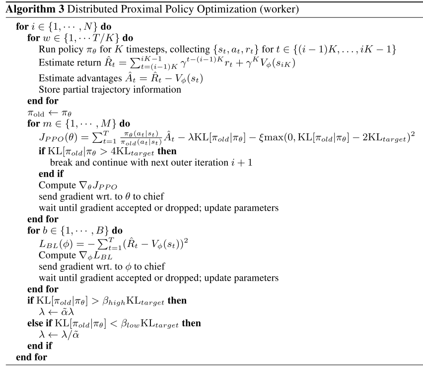
Experiments indicates that averaging gradients and applying them synchronously leads to better results than asynchronously in practice.

Generalized Advantage Estimation(GAE)

Challenges:

1. Requires a large number of samples;
2. Difficulty of obtaining stable and steady improvement despite the non-stationarity of the incoming data.
3. credit reward problem in RL (a.k.a distal reward problem in the behavioral literature): long time delay on rewards.

Solution:^[10]

1. Use value functions to reduce the variance of policy gradient estimates at the cost of some bias, with an exponentially-weighted estimator of advantage function that is analogous to TD($\lambda$);
2. Use TRPO for both policy and value function with NNs.

Advantage function estimation

The advantage has the form:

$$\begin{align} \mathbb{E}_{s_{t+1}} \left[ \delta_t^{V^{\pi,\gamma}} \right] & = \mathbb{E}_{s_{t+1}} [r_t + \gamma V^{\pi, \gamma} (s_{t+1}) - V^{\pi,\gamma}(s_t)] \\ &= \mathbb{E}_{s_{t+1}} [Q^{\pi, \gamma} (s_t, a_t) - V^{\pi, \gamma}(s_t)] \\ &= A^{\pi, \gamma} (s_t, a_t) \end{align}$$

Now take the form of $k$ of $\delta$ terms, denoted by $\hat{A}_t^{(k)}$:

$$\begin{align} &\hat{A}^{(1)}_t := \delta_t^V & = -V(s_t) + r_t + \gamma V(s_{t+1}) \\ &\hat{A}^{(2)}_t := \delta_t^V + \gamma \delta_{t+1}^V & = -V(s_t) + r_t + \gamma r_{t+1} + \gamma^2 V(s_{t+2}) \\ &\hat{A}^{(3)}_t := \delta_t^V + \gamma \delta_{t+1}^V + \gamma^2 \delta_{t+2}^V & = -V(s_t) + r_t + \gamma r_{t+1} + \gamma^2 r_{t+2} + \gamma^3 V(s_{t+3}) \\ & \cdots & \cdots\\ & \hat{A}_t^{(k)} := \sum_{l=0}^{k-1} \gamma^l \delta_{t+1}^V & = - V(s_t) + r_t + \gamma r_{t+1} + \cdots + \gamma^{k-1} r_{t+k-1} + \gamma^kV(s_{t+k}) \end{align}$$

With $k \rightarrow \infty$, the bias generally becomes smaller:

$$\hat{A}^{(\infty)}_t = \sum_{l=0}^\infty \gamma^l \delta_{t+1}^V = -\underbrace{V(s_t)}_\text{value function} + \underbrace{\sum_{l=0}^\infty \gamma^l r_{t+1}}_\text{empirical returns}$$

which is simply the empirical returns minus the value function baseline.

GAE

GAE is defined as the exponentially-weighted average of these $k$-step estimators:

$$\begin{align} \hat{A}_t^{\text{GAE}(\gamma,\lambda)} & := (1-\lambda)(\hat{A}_t^{(1)} + \lambda \hat{A}_t^{(2)} + \lambda^2 \hat{A}_t^{(3)} + \cdots ) \\ & = (1-\lambda) \big(\delta_t^V + \lambda (\delta_t^V + \gamma \delta_{t+1}^V) + \lambda^2 (\delta_t^V + \gamma \delta_{t+1}^V + \gamma^2 \delta_{t+2}^V) + \cdots \big) \\ & = (1-\lambda) \big( \delta_t^V (1+\lambda + \lambda^2 + \cdots) + \gamma \delta_{t+1}^V (\lambda + \lambda^2 + \lambda^3 + \cdots) + \gamma^2 \delta_{t+2}^V (\lambda^2+\lambda^3+\lambda^4+\cdots) + \cdots \big) \\ & = (1-\lambda) \big( \delta_t^V (\frac{1}{1-\lambda}) + \gamma \delta_{t+1}^V (\frac{\lambda}{1-\lambda}) + \gamma^2 \delta_{t+2}^V (\frac{\lambda^2}{1-\lambda}) + \cdots \big) \\ & = \sum_{l=0}^\infty (\gamma \lambda)^l \delta_{t+1}^V \end{align}$$

Now consider two special cases:

• when $\lambda \rightarrow 0$: $$\text{GAE}(\gamma, 0) \quad \hat{A}_t := \delta_t = r_t + \gamma V(s_{t+1}) - V(s_t)$$
• when $\lambda \rightarrow 1$: $$\text{GAE}(\gamma, 1) \quad \hat{A}_t := \sum_{t=0}^\infty \gamma^l \delta_{t+l} = \sum_{l=0}^\infty \gamma^l r_{t+1} - V(s_t)$$

It shows that GAE($\gamma,1$) has high variance due to the sum of terms; GAE($\gamma,0$) induces bias but with lower variance. The GAE with $\lambda \in (0,1)$ reaches a tradeoff between the bias and variance.

Interpretation as Reward Shaping

• Reward shaping refers to the following reward transformation of MDP:

  $$\tilde{r}(s,a,s') = r(s,a,s') + \gamma \Phi(s') - \Phi(s)$$

  where $\Phi: \mathcal{S} \rightarrow \mathbb{R}$ is an arbitrary scalar-valued function on the state space.

• Let $\tilde{Q}^{\pi, \gamma}$, $\tilde{V}^{\pi, \gamma}$, $\tilde{A}^{\pi, \gamma}$ be the value and advatage functions of the transformed MDP:

  $$\tilde{Q}^{\pi, \gamma} (s,a) = Q^{\pi, \gamma} (s,a) - \Phi(s)$$ $$\tilde{V}^{\pi, \gamma} (s,a) = V^{\pi, \gamma} (s,a) - \Phi(s)$$ $$\tilde{A}^{\pi, \gamma} (s,a) = \big(Q^{\pi, \gamma} (s,a) - \Phi(s) \big) -\big( V^{\pi, \gamma} (s,a) - \Phi(s) \big) = A^{\pi, \gamma} (s,a)$$

Let $\Phi = V$, then

$$\sum_{l=0}^\infty (\gamma \lambda)^l \tilde{r}(s_{t+l}, a_t, s_{t+l+1}) = \sum_{l=0}^\infty (\gamma \lambda)^l \delta_{t+l}^V = \hat{A}_t^{\text{GAE}(\gamma, \lambda)}$$

Value function estimation

Constrain the average KL divergence between the previous value function and new value function to be smaller than $\epsilon$:

$$\begin{align} \underset{\phi}{\text{minimize}} & \quad \sum_{n=1}^N ||V_\phi(s_n)- \hat{V}_n ||^2 \\ s.t & \quad \frac{1}{N}\sum_{n=1}^N \frac{||V_\phi(s_n)- V_{\phi_\text{old}}(s_n)||^2}{2\sigma^2} \le \epsilon \end{align}$$

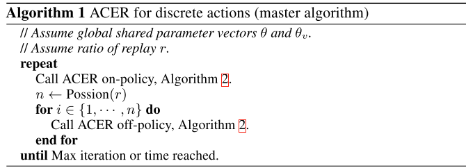
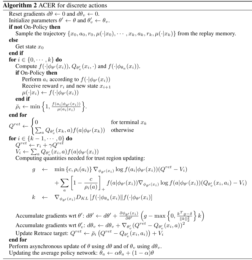
Actor-Critic with Experience Replay(ACER)

Actor-Critic with Experience Replay(ACER)^[12] employs truncated importance sampling with bias correction, stochastic dueling network architectures, and a new TRPO method.

Importance weight truncation with bias correction

$$\hat{g}^\text{ACER}_t = \bar{\rho}_t \nabla_\theta \log \pi_\theta (a_t \vert x_t) [Q^\text{retrace}(x_t,a_t) - V_{\theta_v}(x_t)] + \mathbb{E}\big( [\frac{\rho_t(a) - c}{\rho_t(a)}]_+ \nabla_\theta \log \pi_\theta (a \vert x_t) [Q_{\theta_v}(x_t, a) - V_{\theta_v}(x_t)] \big)$$

where $\bar{\rho}_t = \min(c,\rho_t)$, with importance weight $\rho_t = \frac{\pi(a_t \vert x_t)}{\mu (a_t \vert x_t)}$

Efficient TRPO

ACER maintains an average policy network $\phi_{\theta_a}$ that represents a running average of past policies and forces the updated policy to not deviate far from the average.

Update the parameter $\theta_a$ of the average policy net work “softly” after each update:

$$\theta_a \leftarrow \alpha \theta_a + (1-\alpha)\theta$$

The policy gradient w.r.t $\phi$:

$$\hat{g}^\text{ACER}_t = \bar{\rho}_t \nabla_{\phi_\theta(x_t)} \log \pi_\theta (a_t \vert \phi_\theta (x)) [Q^\text{retrace}(x_t,a_t) - V_{\theta_v}(x_t)] + \mathbb{E}\big( [\frac{\rho_t(a) - c}{\rho_t(a)}]_+ \nabla_{\phi_\theta(x_t)} \log \pi_\theta (a \vert \phi_\theta (x)) [Q_{\theta_v}(x_t, a) - V_{\theta_v}(x_t)] \big)$$

ACKTR

Soft Q-learning

Soft Q-learning(SQL) expresses the optimal policy via Boltzmann distribution (a.k.a Gibbs distribution).

• Soft Q-learning fomulates a stochastic policy as a (conditional) energy-based model (EBM), with the energy function corresponding to the “soft” Q-function obtained when optimizing the maximum entropy objective.
• “The entropy regularized actor-critic algorithms can be viewed as approaximate Q-learning methods, with the actor serving the role of an approimate sampler from an intrctable posterior” ^[14].

Contributions:

1. Improved exploration performance is with multi-modal reward landscapes, where conventional deterministic or unimodal methods are at high risk of falling into suboptimal local optima.
2. Stochastic energy-based policies can provide a much better initialization for learning new skills than either random policies or policies pretrained with maximum expected reward objectives.

Maximum Entropy RL

• Conventional RL objectives to learn a policy $\pi(\pmb{a}_t \vert \pmb{s}_t)$: $$\pi^*_\text{std} = \arg \max_\pi \sum_t \mathbb{E}_{(s_t, a_t) \sim \rho_\pi} [r(s_t, a_t)]$$
• Maximum entropy RL augments the entropy term to maximize its entropy at each visited state: $$\pi^*_\text{std} = \arg \max_\pi \sum_t \mathbb{E}_{(s_t, a_t) \sim \rho_\pi} [r(s_t, a_t) + \alpha \mathcal{H} (\pi(\cdot \vert s_t)) ]$$ where $\alpha$ is used to determine the relative importance of entropy and reward.

Energy-based models (EBM)

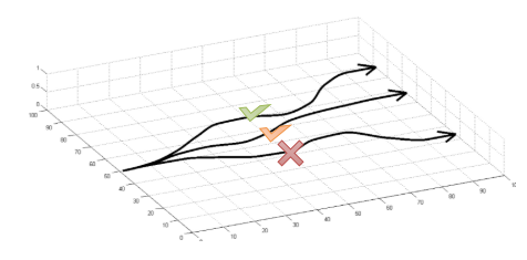
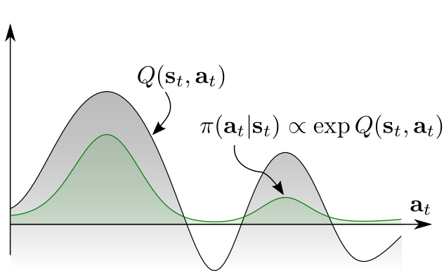
As the figure below, the conventional RL specifies a unimodal policy distribution, centered at the maimal Q-value and extending toe the neighboring actions to provide noise for exploration (as red distribution). The exploration is biased towards the upper mode, RL ignores the lower mode completely.^[15]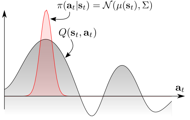

To ensure the agent to explore all promising states while prioritizing the more promising mode, Soft Q-learning definesthe policy w.r.t exponentiated Q-values (see green distribution):

$$\pi(a_t \vert s_t) \propto \exp(-\mathcal{Q}(s_t, a_t))$$

where $\mathcal{Q}$ is an energy function, that could be represented by NNs.

Soft value functions

The soft Bellman equation:

$$Q(s_t, a_t) = \mathbb{E} \left[ r_t + \gamma \text{softmax}_a Q(s_{t+1}, a) \right]$$

where

$$\text{softmax}_a f(a) := \log \int_a \exp f(a) da$$

The soft Q-function is:

$$Q^*_\text{soft} (s_t, a_t) = r_t + \mathbb{E}_{(s_{t+1,\cdots}) \sim \rho_\pi} \mathcal{H} (\pi^*_\text{MaxEnt}(\cdot \vert s_{t+l}))$$

The soft value function:

$$V^*_\text{soft} (s_t) = \alpha \log \int_\mathcal{A} \exp \big( \frac{1}{\alpha} Q^*_\text{soft}(s_t, a') \big) da'$$

Then the optimal policy is:

$$\begin{align} \pi^*_\text{MaxEnt}(a_t \vert s_t) &= \exp \big( \frac{1}{\alpha} (Q^*_\text{soft} (\underbrace{s_t, a_t) - V^*_\text{soft}(s_t)}_{\text{advantage function}}) \big) & \\ &=\frac{\exp(\frac{1}{\alpha}Q^*_\text{soft}(s_t,a_t))}{\int_\mathcal{A} \exp(\frac{1}{\alpha} Q^*_\text{soft}(s_t,a')) da'} & \\ &= \frac{\exp(\frac{1}{\alpha}Q^*_\text{soft}(s_t,a_t))}{\exp(\frac{1}{\alpha}V^*_\text{soft}(s_t))} & \end{align}$$

Proofs

• Define the optimal policy with the EBM form: $$\pi^*(a \vert s) = \frac{\exp(Q(s,a))}{Z}$$ where $Z$ is the sum of the numerator.
• Minimize the KL divergence:

$$\begin{align} \min \mathbb{KL} (\pi || \tilde{\pi}) & = \sum \pi(a \vert s) \log \frac{\pi(a \vert s)}{\tilde{\pi}(a \vert s)} & \\ & = \underbrace{\sum \pi(a \vert s) \log \pi(a \vert s)}_{- \mathbb{H}(\cdot \vert \pi)} - \sum \pi(a \vert s) \log \tilde{\pi}(a \vert s) & \text{expand KL divergence}\\ &= - \mathbb{H}(\cdot \vert \pi) - \sum \pi(a \vert s) \left[ Q(s_t,a_t) - \underbrace{log Z}_{V(s)} \right] \\ \text{here, } & & \\ V(s) & = \log Z & \\ & = \log \int_\mathcal{A} \exp \left( \frac{1}{\alpha} Q(s',a') da' \right) \end{align}$$

Soft Q-learning

• Soft Bellman-backup $$\begin{align*} Q_\text{soft}(s_t,a_t) &\leftarrow r_t+\gamma\mathbb{E}_{s_{t+1}\sim p_s}[V_\text{soft}(s_{t+1})] \\ V_\text{soft}(s_t) &\leftarrow \alpha\log\int_\mathcal{A} \exp\left( \frac{1}{\alpha} Q_\text{soft}(s_t,a') \right)\mathrm{d}a' \end{align*}$$

This cannot be performed exactly in countinuous or large state and action spaces. Sampling from the energy-based model is intractable in general.

Sampling

Importance sampling

$$V^\theta_\text{soft} (s_t) = \alpha \log \mathbb{E}_{q_{a'}} \left[ \frac{\exp(\frac{1}{\alpha} Q_\text{soft}^\theta(s_t, a') )}{q_{a'}(a')} \right]$$

where $q_{a'}$ can be an arbitrary distribution over the action space.
It can also be equivalent as minimizing:

$$J_Q(\theta) = \mathbb{E}_{s_t \sim q_{s_t}, a_t \sim q_{a_t}} \left[ \frac{1}{2} \big( \hat{Q}^{\bar{\theta}}_\text{soft} (s_t,a_t) - Q_\text{soft}^\theta (s_t,a_t) \big)^2 \right]$$

where $\hat{Q}^{\bar{\theta}}_\text{soft} (s_t, a_t) = r_t + \gamma \mathbb{E}_{s_{t+1} \sim p_s} [V_\text{soft}^{\bar{\theta}}(s_{t+1})]$ is the target $Q$-value.

Stein Variational Gradient Descent (SVGD)

• How to approximately sample from the soft Q-funtion?
  1. MCMC based sampling
  2. learn a stochastic sampling network trained to output approximate samples from the target distribution

Soft Q-learning applies the sampling network based on Stein variational gradient descent (SVGD) and amortized SVGD.

1. Learn a state-conditioned stochastic NN $a_t = f^\phi(\xi; s_t)$ that maps noise samples $\xi$ drawn from an arbitrary distribution into unbiased action samples from the target EBM of $Q_\text{soft}^\theta$.
2. The induced distribution of the actions $\pi^\phi (a_t \vert s_t)$ approximates the energy-based distribution w.r.t KL divergence: $$J_\pi(\phi^\phi \big(\cdot \vert s_t) || \exp(\frac{1}{\alpha} (Q_\text{soft}^\theta(s_t, \cdot) - V_\text{soft}^\theta ) ) \big)$$
3. SVGD provides the most greedy directions as a functional: $$\Delta f^\phi(\cdot ; s_t) = \mathbb{E}_{a_t \sim \pi^\phi} \big[\kappa (a_t, f^\phi(\cdot;s_t)) \nabla_{a'}Q^\theta_\text{soft}(s_t, a') |_{a'=a_t} + \alpha \nabla_{a'}\kappa (a',f^\phi(\cdot;s_t))|_{a'=a_t} \big]$$ Update the policy networks: $$\frac{\partial J_\pi (\phi; s_t)}{\partial \phi} \propto \mathbb{E}_\xi \left[ \Delta f^\phi(\xi; s_t)\frac{\partial f^\phi (\xi; s_t)}{\partial \phi} \right]$$

Algorithms

$\mathcal{D} \leftarrow$ empty replay memory
Assign target parameters: $\bar{\theta} \leftarrow \theta$, $ \bar{\phi} \leftarrow \phi $

1. for each epoch:
   1. for each t do:
      1. Collect experience
         Sample an action for $s_t$ using $f^\phi$: $a_t f^\phi(\xi;s_t)$ where $\xi \sim (0; I)$
         Sample next state from the environment: $s_{t+1} \sim p_s(s_{t+1} \vert s_t, a_t)$
         Save the new experience in the replay memory: $\mathcal{D} \leftarrow \mathcal{D} \cup \{ (s_t,a_t,r(s_t,a_t), s_{t+1}) \}$
      2. Sample a mini-batch from the replay memory $\{(s_t^{(i)}, a_t^{(i)}, r_t^{(i)},s_{t+1}^{(i)})\}_{i=0}^N \sim \mathcal{D}$
      3. Update the soft Q-function parameters:
         Sample $\{ a^{(i,j)} \}_{j=0}^M \sim q_{a'}$ for each $s_{t+1}^{(i)}$
         Compute empirical soft values $\hat{V}_\text{soft}^\bar{\theta} (s_{t+1}^{(i)})$ in $$V^\theta_\text{soft} (s_t) = \alpha \log \mathbb{E}_{q_{a'}} \left[ \frac{\exp(\frac{1}{\alpha} Q_\text{soft}^\theta(s_t, a') )}{q_{a'}(a')} \right]$$ Compute empirical gradient $\hat{\nabla}_\theta J_Q$ of $$J_Q(\theta) = \mathbb{E}_{s_t \sim q_{s_t}, a_t \sim q_{a_t}} \left[ \hat{Q}^{\bar{\theta}}_\text{soft} (s_t,a_t) - Q_\text{soft}^\theta (s_t,a_t)^2 \right]$$ Update $\theta$ according to $\hat{\nabla}_\theta J_Q$ using Adam.
      4. Update policy
         Sample $\{ \xi^{(i,j)} \}_{j=0}^{M} \sim \mathcal{N} (\pmb{0},\pmb{I})$ for each $s_t^{(i)}$
         Compute actions $a_t^{(i,j)}= f^\phi(\xi^{(i,j)}, s_t^{(i)})$
         Compute $\Delta f^\phi$ using empirical estimate of $$\Delta f^\phi(\cdot ; s_t) = \mathbb{E}_{a_t \sim \pi^\phi} \big[\kappa (a_t, f^\phi(\cdot;s_t)) \nabla_{a'}Q^\theta_\text{soft}(s_t, a') |_{a'=a_t} + \alpha \nabla_{a'}\kappa (a',f^\phi(\cdot;s_t))|_{a'=a_t} \big]$$ Compute empirical estimtate of $\hat{\nabla}_\phi J_\pi$ of $$\frac{\partial J_\pi (\phi; s_t)}{\partial \phi} \propto \mathbb{E}_\xi \left[ \Delta f^\phi(\xi; s_t)\frac{\partial f^\phi (\xi; s_t)}{\partial \phi} \right]$$ Update $\phi$ according to $\hat{\nabla}_\phi J_\pi$ using Adam
   2. If epoch $%$ update_interval == 0:
      $\bar{\theta} \leftarrow \theta, \quad \bar{\phi} \leftarrow \phi $

Benefits

• Better exploration. SQL provides an implicit exploration stategy by assgining each action a non-zero probability, shaped by the current belief about its value, effectively combining exploration and exploitation in a natural way.^[15]
• Fine-tuning maximum entropy policies: general-to-specific transfer.Pre-train policies for general purpose tasks, then use them as templates or initializations for more specific tasks.
• Compositionality. Compose new skills from existing policies—even without any fine-tuning—by intersecting different skills.^[15]

• Robustness. Maximum entropy formulation encourages to try all possible solutions, the agents learn to explore a large portion of the state space. Thus they learn to act in various situations, more robust against perturbations in the environment.

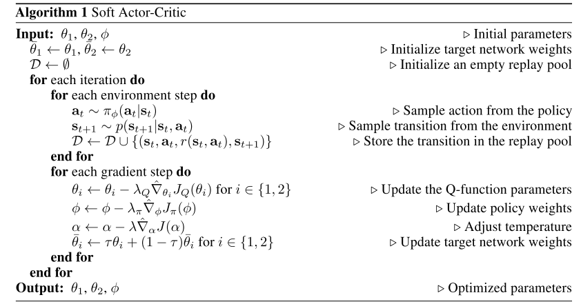
Soft Actor-Critic(SAC)

Soft Actor-Critic (SAC)^[13] is an off-policy actor-critic algorithm based on the maximum entropy framework. Like SQL, SAC augments the conventional RL objectives with a maximum entropy objective:

$$J(\pi) = \sum_{t=0}^T \mathbb{E}_{(s_t,a_t) \sim \rho_\pi} \left[ r(s_t,a_t) + \alpha \mathcal{H}(\pi(\cdot \vert s_t)) \right]$$

where the $\alpha$ determines the relative importance of the entropy term against the reward, and thus controls the stochasticity of the optimal policy.

The maximum entropy terms

1. Encourage to explore more widely, while giving up on clearly unpromising avenues;
2. Capture multiple modes of near-optimal behavior.
3. Improve learning speed and exploration.

Soft policy iteration

Policy evaluation

The soft-Q value of the policy $\pi$:

$$\tau^\pi Q(s_t,a_t) \triangleq r(s_t,a_t) + \gamma \mathbb{E}_{s_{t+1} \sim p} [V(s_{t+1}) ]$$

where the soft state value function:

$$V(s_t) = \mathbb{E}_{a_t \sim \pi} [Q(s_t, a_t) - \log \pi(a_t \vert s_t)]$$

Policy Improvement

For each state, we update the policy according to:

$$\pi_\text{new} = \arg \min_{\pi'} D_\mathbb{KL}(\pi'(\cdot \vert s_t) || \frac{\exp(Q^\text{old}(s_t, \cdot))}{Z^{\pi_\text{old}(s_t)}})$$

where the partitioning function $Z^{\pi_\text{old}}(s_t)$ normalizes the distribution.

SAC

Consider a parameterized state value function $V_\Psi (s_t)$, soft Q-function $Q_\theta (s_t,a_t)$ and a tractable policy $\pi_\phi (a_t \vert s_t)$.

The soft value function is trained to minimize the squared residual error:

$$J_{V(\Psi)} = \mathbb{E}_{s_t \sim \mathcal{D}} \left[ \frac{1}{2} \big(V_\Psi (s_t)-\mathbb{E}_{a_t \sim \pi_\phi} [Q_\theta (s_t, a_t)+ \log \pi_\phi (a_t \vert s_t)] \big) \right]$$

The soft Q-function can be trained to minimize the soft Bellman residual:

$$J_Q (\theta) = \mathbb{E}_{(s_t,a_t) \sim \mathcal{D}} \left[ \frac{1}{2}\big( Q_\theta(s_t,a_t)-\hat{Q}(s_t,a_t) \big)^2 \right]$$

with

$$\hat{Q}(s_t, a_t) = r(s_t, a_t) + \gamma \mathbb{E}_{s_{t+1}\sim p} [V_\bar{\psi}(s_{t+1})]$$

The policy can be optimized by the expected KL-divergence:

$$J_\pi(\phi) = \mathbb{E}_{s_t \sim \mathcal{D}} \left[ D_\text{KL} \big( \pi_\phi(\cdot \vert s_t) || \frac{\exp(Q_\theta(s_t,\cdot))}{Z_\theta(s_t)} \big) \right]$$

Minimizing $J_\pi$ with reparameterization trick.

• Reparameterize the policy with an NN transformation: $$a_t = f_\phi(\epsilon_t; s_t)$$ where $\epsilon$ is an input noise vector, sampled from some fixed distribution.

• Rewrite the previous objective as:

  $$J_\pi(\phi) = \mathbb{E}_{s_t \sim \mathcal{D}, \epsilon_t \sim \mathcal{N}} [\log \pi_\phi (f_\phi(\epsilon_t;s_t) \vert s_t) - Q_\theta(s_t, f_\phi(\epsilon_t;s_t))]$$

• Employ two Q-functions to mitigate positive bias in the policy improvement step, using the minimum of the Q-functions for the value gradient and policy gradient.

Automatically adjusted temperature

SAC is brittle w.r.t the temperature parameter. Choosing the optimal temperature $\alpha$ is non-trival, and the temperature needs to be tuned for each task. ^[17]

SAC finds a stochastic policy with maximal expected return that satisfies a minimum expected entropy constraint.

$$\max_{\pi_{o:T}} \mathbb{E}_{\rho_\pi} \left[ \sum_{t=0}^T r(s_t,a_t) \right] \quad s.t. \quad \mathbb{E}_{(s_t,a_t)\sim \rho_\pi} [- \log(\pi_t(a_t \vert s_t))] gleq \mathcal{H} \forall t$$

where $\mathcal{H}$ is a desired minimum expected entropy.

• Rewite the objective as an iterated maximization $$\max_{\pi_0} \big( \mathbb{E} [r(s_0,a_0)] + \max_{\pi_1}\big( \mathbb{E}[\cdots] + \max_{\pi_T} \mathbb{E}[r(s_T,a_T)] \big) \big)$$
• Finally we get: $$\alpha_t^* = \arg\min_{\alpha_t} \mathbb{E}_{a_t \sim \pi_t^*} [-\alpha_t \log \pi_t^* (a_t \vert s_t; \alpha_t) -\alpha_t \bar{\mathcal{H}}]$$

Algorithms

Update $\alpha$ with following objective:

$$J(\alpha) = \mathbb{E}_{a_t \sim \pi_t} [-\alpha \log \pi_t(a_t \vert s_t) -\alpha \bar{\mathcal{H}}]$$

Deterministic Policy Gradient (DPG)

Deep DPG (DDPG)

Distributed Distributional DDPG(D4PG)

Multi-Agent DDPG(MADDPG)

Twin Delayed Deep Deterministic PG(TD3)

References

---

1. 1.Mnih, V., Badia, A.P., Mirza, M.P., Graves, A., Lillicrap, T.P., Harley, T., Silver, D., & Kavukcuoglu, K. (2016). Asynchronous Methods for Deep Reinforcement Learning. ICML. ↩
2. 2.Policy gradient algorithms #A3C ↩
3. 3.- Actor: updates the policy parameters $\theta$ for $\pi_\theta(a \vert s)$ in the direction suggested by the critic. - Critic: updates the value function parameter $w$ and could be action-value $Q_w(a \vert s)$ or state-value $V_w(s)$ ↩
4. 3.Sutton, R.S., & Barto, A.G. (1988). Reinforcement Learning: An Introduction. IEEE Transactions on Neural Networks, 16, 285-286. ↩
5. 4.A2C ↩
6. 5.Schulman, J., Levine, S., Abbeel, P., Jordan, M.I., & Moritz, P. (2015). Trust Region Policy Optimization. ICML. ↩
7. 6.TRPO blog 1 ↩
8. 7.TRPO blog 2 ↩
9. 8.Schulman, J., Wolski, F., Dhariwal, P., Radford, A., & Klimov, O. (2017). Proximal Policy Optimization Algorithms. ArXiv, abs/1707.06347. ↩
10. 9.Heess, N., Dhruva, T., Sriram, S., Lemmon, J., Merel, J., Wayne, G., Tassa, Y., Erez, T., Wang, Z., Eslami, S.M., Riedmiller, M.A., & Silver, D. (2017). Emergence of Locomotion Behaviours in Rich Environments. ArXiv, abs/1707.02286. ↩
11. 10.Schulman, J., Moritz, P., Levine, S., Jordan, M.I., & Abbeel, P. (2016). High-Dimensional Continuous Control Using Generalized Advantage Estimation. CoRR, abs/1506.02438. ↩
12. 11.Wu, Y., Mansimov, E., Grosse, R. B., Liao, S., & Ba, J. (2017). Scalable trust-region method for deep reinforcement learning using kronecker-factored approximation. In Advances in neural information processing systems (pp. 5279-5288). ↩
13. 12.Wang, Z., Bapst, V., Heess, N., Mnih, V., Munos, R., Kavukcuoglu, K., & de Freitas, N. (2016). Sample efficient actor-critic with experience replay. arXiv preprint arXiv:1611.01224. ↩
14. 13.Haarnoja, T., Zhou, A., Abbeel, P., & Levine, S. (2018). Soft actor-critic: Off-policy maximum entropy deep reinforcement learning with a stochastic actor. arXiv preprint arXiv:1801.01290. ↩
15. 14.Haarnoja, T., Tang, H., Abbeel, P., & Levine, S. (2017, August). Reinforcement learning with deep energy-based policies. In Proceedings of the 34th International Conference on Machine Learning-Volume 70 (pp. 1352-1361). JMLR. org. ↩
16. 15.Soft Q-learning, UC Berkeley blog ↩
17. 16.Notes on the Generalized Advantage Estimation Paper ↩
18. 17.Haarnoja, T., Zhou, A., Hartikainen, K., Tucker, G., Ha, S., Tan, J., ... & Levine, S. (2018). Soft actor-critic algorithms and applications. arXiv preprint arXiv:1812.05905. ↩