Efficient Large-Scale Distributed Training

A note of distributed training methods for large neural models.

Training Parallelism

Data Parallelism

Data parallelism (DP) is a technique where we replicate the entire model’s parameters across multiple devices. During training, the mini-batch of data is partitioned evenly across all participating devices. This means that each device, or DP process, operates on a distinct subset of the data samples.

The training process in data parallelism involves each device executing its own forward and backward propagation. This computes the gradients based on the subset of data it has been assigned. Once the gradients are computed, they are averaged across all devices to ensure a consistent update to the model parameters.

Model Parallelism

Model Parallelism (MP)^[1] offers a way to scale neural network training beyond the memory limitations of a single device by distributing the model’s computation across multiple processes. This strategy is particularly useful for large transformer models that would otherwise be too large to fit on a single GPU.

Tensor-level Model Parallelism (MP) divides the model’s computation vertically among different devices or processes.

MLP

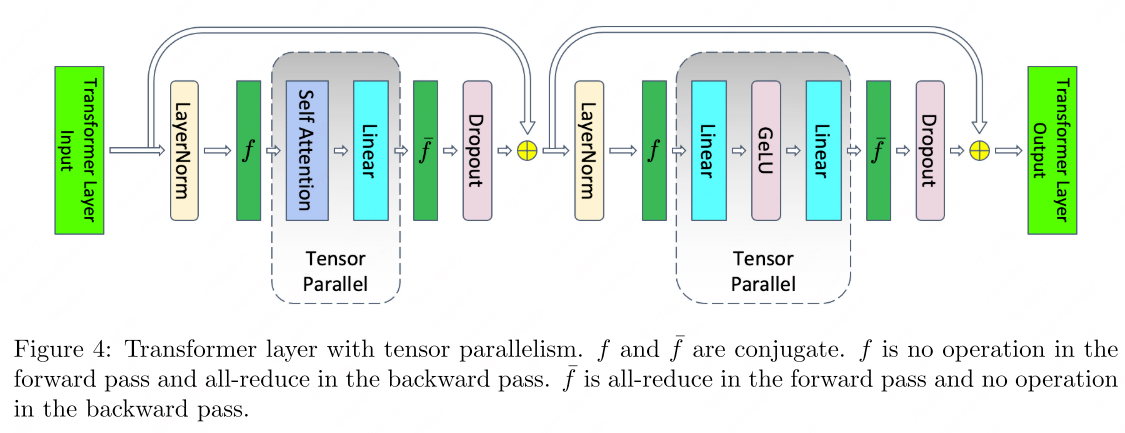
To illustrate how MP works, let’s consider the standard Multilayer Perceptron (MLP) block within a transformer model, which is represented by the following equations:

\begin{equation}
Y=\mathrm{GeLU}(XA)
\end{equation}

\begin{equation}
Z=\mathrm{Dropout}(YB)
\end{equation}

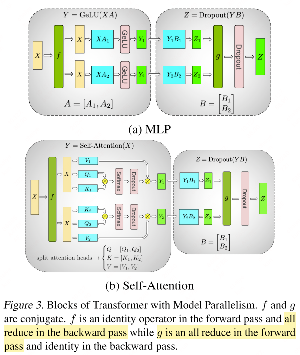
For the MLP block, tensor-level MP splits the weight matrix $A$ into columns $A = [A_1, A_2]$. By partitioning
$A$, the GeLU activation function can be applied independently to the outputs of each partitioned matrix multiplication (GEMM):

\begin{equation}
[Y_1,Y_2]=[\text{GeLU}(XA_1),\text{GeLU}(XA_2)]
\end{equation}

The subsequent GEMM, represented by matrix $B$, is split along its rows. This enables direct input from the GeLU activations without the need for inter-process communication, as depicted in the figure above.

Self-Attention

The self-attention mechanism is a cornerstone of transformer models, described by the following equation:

\begin{equation}
\text{Attention}(X,Q,K,V)=\text{softmax}(\frac{(XQ)(XK)^\top}{\sqrt{d_k}})XV
\end{equation}

For self-attention black, MP partitions the GEMMs for key ($K$), query ($Q$), and value ($V$) matrices along their columns. This allows for the matrix multiplication of each attention head to be distributed across individual GPUs. The output linear layer’s GEMM is then split along its rows, facilitating an efficient transformer layer that requires only two all-reduce operations in both the forward and backward passes.

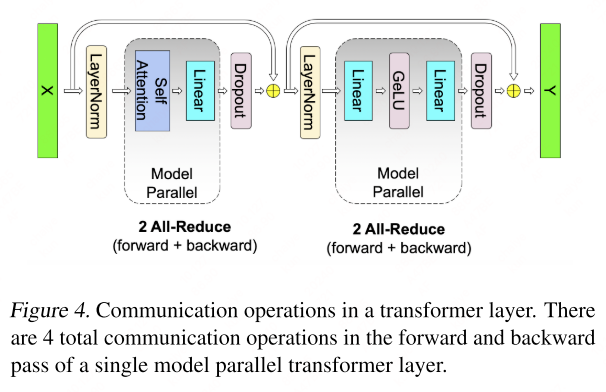
When it comes to components like dropout, layer normalization, and residual connections, MP adopts a different approach. Instead of splitting these operations, MP replicates their computations across GPUs. This ensures that the output of the MP region can seamlessly integrate with these operations without additional device communication.

To achieve this, MP maintains duplicate copies of the layer normalization parameters on each GPU. As a result, each GPU can perform dropout and residual connection operations independently, taking the output from the MP region and processing it locally.

Model Parallelism, by partitioning the model’s computation across multiple devices, effectively enables training of large-scale transformer models that would otherwise exceed the memory capabilities of a single device. Careful consideration of how operations like dropout and layer normalization are handled ensures that MP remains efficient without compromising the integrity of the model’s training.

Pipeline Parallelism

Pipeline Parallelism (PP)^[5][6][2] splits the forward and backward pipelines into multiple stages, each assigned to a different device, and data flows through these stages sequentially, enabling efficient utilization of resources and faster training of large models.

GPipe

GPipe^[5] pipelines different sub-sequences of layers on separate accelerators, where consecutive groups of layers can be partitioned into cells. GPipe divides the input mini-batch into smaller micro-batches, enabling different accelerators to work on different micro-batches simutaneously.

Pipeline Bubble (bubble size): Given the PP stages $p$ (PP degree), the sequence of $L$ layers can be partitioned into $p$ composite layers, or cells. The numbder of micro-batches in a batch as $m$. The PP bubble consists of $p-1$ forward passes at the start of a batch, and $p-1$ backward passes at the end. Thus, the pipeline bubble size (bubble time fraction) is defined as:

$$\begin{equation} \text{Bubble time fraction (bubble size)}=1- \frac{mp}{(m+p-1)d}=\frac{p-1}{m+p-1}. \end{equation}$$

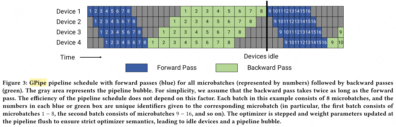
When $m > 4d$, the bubble overhead is negligible.

PipeDream

PipeDream^[6] revolutionizes the efficiency of pipeline parallelism in deep learning with its one-forward-one-backward (1F1B) strategy. This approach guarantees that no GPU remains idle during the steady state, thereby ensuring continuous forward progress with each minibatch. It achieves this by immediately initiating the backward pass for a minibatch as soon as its forward pass is completed.

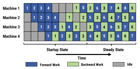
The 1F1B strategy interleaves the forward and backward computations at the minibatch level. This tight coupling of passes optimizes the use of GPU resources and accelerates the learning process, as each minibatch benefits from immediate backward propagation, leading to quicker gradient updates and model improvements.

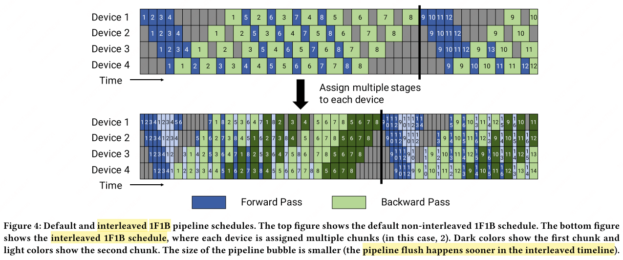
For interleaved schedules in PipeDream, it allows each device to handle multiple subsets of layers, referred to as model chunks, rather than being restricted to a single, contiguous block of layers. As a result, each device in the pipeline is responsible for multiple pipeline stages, dramatically increasing the efficiency of the computation distribution.

The figure above illustrates that if each device manages $v$ stages, or model chunks, the time required for processing a minibatch through both the forward and backward passes is reduced to $\frac{1}{v}$ of the time it would have previously taken. Consequently, this reduction in processing time diminishes the pipeline bubble—the period when some GPUs might otherwise be idle—resulting in a more streamlined and efficient training process. The bubble size can be quantified as follows:

$$\begin{equation} \text{Bubble time fraction (bubble size)}=\frac{1}{v} \cdot \frac{p-1}{m+p-1}. \end{equation}$$

Here, $d$ represents the degree of pipeline parallelism (number of devices), and $m$ is the number of microbatches in a batch.

Sequence Parallelism

Model parallelism (MP) retains critical components like layer normalization, dropout, and residual connections across the MP group intact. A key insight presented in ^[3] is that in certain regions of transformer blocks, operations are independent along the sequence dimension. SP ^[3] partitions these regions along the sequence dimension for enhanced parallel processing.

Consider the following standard non-parallel block within a transformer layer:

$$\begin{align} Y& =\mathrm{LayerNorm}(X) \\ Z& =\mathrm{GeLU}(YA), \\ W& =ZB, \\ V &=\mathrm{Dropout}(W), \end{align}$$

Sequence parallelism splits the input to the layer normalization along the sequence dimension: $X=[X_{1}^{s},X_{2}^{s}]$. Consequently, the output of the layer normalization is also parallel along the sequence dimension: $Y=[Y_{1}^{s},Y_{2}^{s}]$. The subsequent linear layer with GeLU activations requires the complete input $Y$, necessitating an all-gather operation. The matrices $A=[A_{1}^{c},A_{2}^{c}]$ and $B=[B_{1}^{r},B_{2}^{t}]$ are partitioned along their columns and rows, respectively. This partitioning strategy helps to minimize communication overhead and allows us to compute $W_1$ and $W_2$ independently. Afterwards, $W=W_1+W_2$ is combined and passed through the dropout layer using reduce-scatter to maintain parallelism along the sequence dimension.

Putting it all together, we articulate the SP processing steps as follows:

$$\begin{align} [Y_{1}^{s},Y_{2}^{s}]& =\mathrm{LayerNorm}([X_{1}^{s},X_{2}^{s}]), \\ \text{Y}& =g(Y_1^s,Y_2^s), \\ [Z_1^h,Z_2^h]& =[\mathrm{GeLU}(YA_{1}^{c}), \mathrm{GeLU}(YA_{2}^{c})], \\ W_{1}& =Z_{1}^{h}B_{1}^{r} \quad W_{2}=Z_{2}^{h}B_{2}^{r}, \\ [W_{1}^{s},W_{2}^{s}]& =\bar{g}(W_1,W_2), \\ [V_{1}^{s},V_{2}^{s}]& =[\mathrm{Dropout}(W_{1}^{s}), \mathrm{Dropout}(W_{2}^{s})]. \end{align}$$

SP divides and conquers the workload along the sequence dimension without compromising the integrity of the underlying operations.

Memory-Efficient Optimizer (ZeRO)

Zero Redundancy Optimizer (ZeRO)^[4] optimizes the memory by removing the memory state redundancies across DP processes by partitioning the model states instead of replicating them. ZeRO-DP has three main statges, corresponding to the partitioning of optimizer states, gradients, and parameters.

1. Optimizer state partitioning ($P_\text{os}$);
2. Add gradient partitioning ($P_\text{os+g}$));
3. Add parameter partitioning ($P_\text{os+g+p}$));

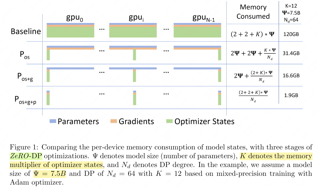
Details refer to https://www.deepspeed.ai/tutorials/zero/.

Pytorch FSDP

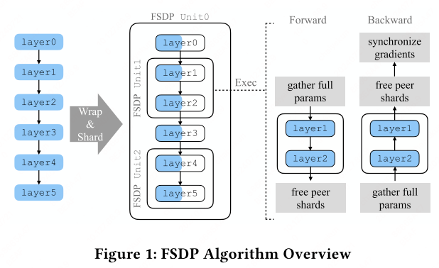
PyTorch Fully Sharded Data Parallel (FSDP)^[8] is designed to accommodate extremely large models that exceed the memory capacity of a single GPU. By decomposing a model instance into smaller fragments, FSDP manages each fragment independently. During the forward and backward computations, FSDP strategically materializes only the unsharded parameters and gradients for one fragment at a time, while keeping the rest of the parameters and gradients in their sharded state.

This resource management means that FSDP only fully materializes the parameters and gradients for a single fragment at any given time, allowing the remaining fragments to remain sharded and thus minimizing memory usage.

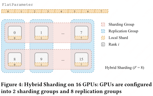
FSDP employs a sharding factor $F$ ato determine the number of ranks over which the parameters are distributed:

1. When $F=1$, FSDP replicates the entire model across all devices, reducing to the conventional Data Parallel (DP) approach, which relies on all-reduce operations for gradient synchronization.
2. For $F=W$,, where $W$ is the global world size, FSDP fully shards the model so that each device maintains only $\frac{1}{W}$ of the total model parameters.
3. When $F \in (1, W)$, FSDP enables hybrid sharding, balancing between replication and full sharding.

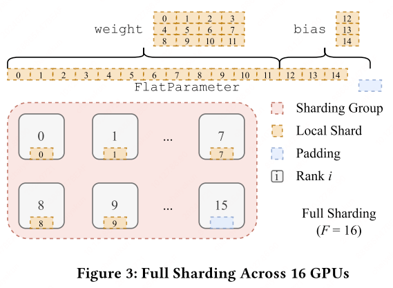
Sharding strategy: flatten-concat-chunk algorithm. FSDP uses a sharding strategy known as the flatten-concat-chunk algorithm. This technique entails organizing all parameters within an FSDP unit into a single contiguous FlatParameter. This FlatParameter, which is a one-dimensional tensor, is created by concatenating and flattening the individual parameters, with padding added as necessary to ensure the size is divisible by the sharding factor $F$. The FlatParameter is then divided into equal-sized chunks, with the number of chunks corresponding to the sharding factor, and each chunk is assigned to a different rank.

By leveraging this strategy, FSDP streamlines communication between the parameters and ensures an even distribution of the model across the ranks. This allows for efficient scaling of model training across multiple GPUs, making it possible to train models that were previously too large to fit in the memory of a single device.

Mixed Precision Training

Mixed precision methods^[9][10] utilize different numerical formats within a single computational workload, optimizing operations by executing them in half-precision (FP16) format. This approach not only accelerates training but also reduces memory usage, allowing for larger models or batch sizes.

During mixed precision training, weights, activations, and gradients are predominantly stored as FP16 to benefit from the reduced precision’s efficiency. However, to maintain the training stability and model quality, an FP32 master copy of weights is kept. This master copy is updated with weight gradients during the optimization step. For each iteration, an FP16 copy of the master weights is used for the forward and backward passes.

Mixed Precision

Mixed precision methods^[9][10] combine the use of different numerical formats in one computational workload.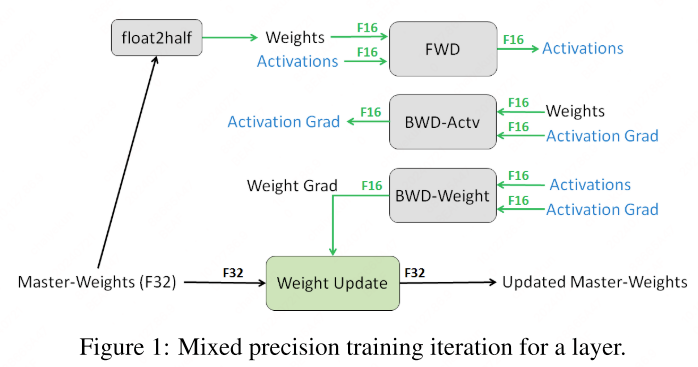

The training procedure for mixed precision training can be summarized as follows:

Mixed precision training:

1. Keep a master copy of weights in full precision (FP32).
2. For each iteration:
   a. Make an FP16 copy of the weights;
   b. Forward propagation (FP16 weights and activations).
   c. Multiply the results loss with the scaling factor $S$.
   d. Backward propagation (FP16 weights, activations, and their gradients).
   e. Multiply (scaling down) the weight gradient with 1/S.
   f. Updating the master weights in FP32, applying necessary adjustments like gradient clipping.

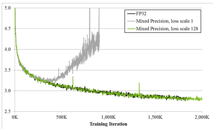
Dynamic loss scaling

This technique involves starting with a large scaling factor and adjusting it dynamically throughout the training process. If no numerical overflow occurs for a predefined number of iterations $N$, the scaling factor $S$ is increased. Conversely, if an overflow is detected, the current weight update is skipped, and $S$ is decreased to prevent future overflows.

Mixed precision training:

1. Maintain a primary copy of weights in FP32.
2. Initialize $S$ to a large value.
3. For each iteration:
   a. Make an FP16 copy of the weights;
   b. Forward propagation (FP16 weights and activations).
   c. Multiply the results loss with the scaling factor $S$.
   d. Backward propagation (FP16 weights, activations, and their gradients).
   e. If there is an inf or nan in weights gradients:

    (1) Reduce S. (2) Skip the weight update and move to the next iteration.

   f. Multiply the weight gradient with 1/S.
   g. Complete the weight update (including gradient clipping, etc.)
   h. If there has not been an inf or nan in the last $N$ iterations, increase $S$.

Implementation:

# Creates model and optimizer in default precision
model = Net().cuda()
optimizer = optim.SGD(model.parameters(), ...)

# Creates a GradScaler once at the beginning of training.
scaler = GradScaler()

for epoch in epochs:
    for input, target in data:
        optimizer.zero_grad()

        # Runs the forward pass with autocasting.
        with autocast(device_type='cuda', dtype=torch.float16):
            output = model(input)
            loss = loss_fn(output, target)

        # Scales loss.  Calls backward() on scaled loss to create scaled gradients.
        # Backward passes under autocast are not recommended.
        # Backward ops run in the same dtype autocast chose for corresponding forward ops.
        scaler.scale(loss).backward()

        # scaler.step() first unscales the gradients of the optimizer's assigned params.
        # If these gradients do not contain infs or NaNs, optimizer.step() is then called,
        # otherwise, optimizer.step() is skipped.
        scaler.step(optimizer)

        # Updates the scale for next iteration.
        scaler.update()

Automatic Mixed Precision (AMP) settings of apex.amp:
opt_level:

• O0: FP32 training

• O1: Mixed precision (recommended). Use a whitelist-blacklist model. Whitelist ops (e.g., tensor core-freindly ops like GEMM and convolutions) are performed in FP16; blacklist ops that benefit from FP32 precision (e.g, softmax) are performaed in F32. O1 uses dynamic loss scaling unless overridden.

• O2: “Almost FP16” Mixed Precision. O2 casts the model weights to FP16, patches the model’s ‘forward’ mothod to cast input data to FP16, keeps batchnorms in FP32, maintains FP32 master weights, update the optimizer’s param_groups so that the optimizer.step acts directly on FP32 weights, and uses dynamic loss scaling. Unlike O1, O2 does not patch Torch functions or Tensor methods.

Property	O0: FP32 Training	O1: Mixed Precision	O2: “Almost FP16” Mixed Precision	O3: FP16 Training
Description	Full FP32 training, useful for establishing an accuracy baseline.	Mixed precision with dynamic casting of operations based on a whitelist-blacklist model. Recommended for typical use.	Almost FP16 training, with model weights and inputs cast to FP16, but BatchNorm and master weights in FP32.	Full FP16 training, useful for establishing a speed baseline. Less stable than O1/O2.
cast_model_type	torch.float32	None (not applicable, model weights remain FP32)	torch.float16 (model weights cast to FP16)	torch.float16 (model weights cast to FP16)
patch_torch_functions	False	True (patches Torch functions and Tensor methods for dynamic FP16/FP32 casting)	False (no patching, explicit control of precision)	False (no patching, explicit control of precision)
keep_batchnorm_fp32	None (not applicable, everything is FP32)	None (not applicable, model weights remain FP32)	True (BatchNorm layers remain in FP32)	False (BatchNorm in FP16, unless overridden with keep_batchnorm_fp32=True)
master_weights	False	None (not applicable, model weights remain FP32)	True (maintains FP32 master weights for optimizer updates)	False (no FP32 master weights)
loss_scale	1.0 (no loss scaling)	"dynamic" (dynamic loss scaling to prevent underflow)	"dynamic" (dynamic loss scaling to prevent underflow)	1.0 (no loss scaling)
Use Case	Baseline for accuracy.	Recommended for typical mixed precision training.	Aggressive mixed precision training with FP16 weights and inputs, but FP32 BatchNorm and master weights.	Baseline for speed. Less stable, useful for comparison with O1/O2.

Key Differences:

• O0: Full FP32 training, no mixed precision. Used for accuracy baselines.
• O1: Dynamic mixed precision with patched Torch functions and Tensor methods. Balances speed and stability.
• O2: Almost FP16 training, with explicit control of precision (no patching). Maintains FP32 BatchNorm and master weights.
• O3: Full FP16 training, no mixed precision. Used for speed baselines but less stable.

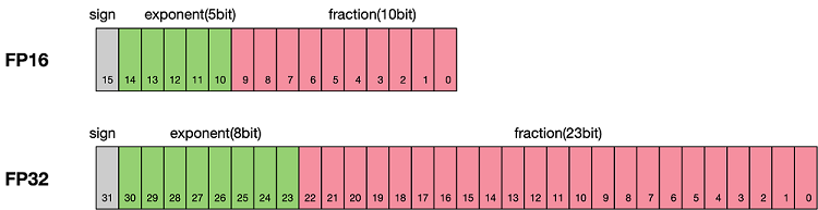
Precision: fp32 (E8M23) fp16 (E5M10)/bf16 (E8M7)/fp8

Memory-efficient methods

CPU Offload

CPU offload: Offloading model states to GPU memory. When GPU memory reaches its capacity, a potential solution is to transfer data that is not immediately required to the CPU, retrieving it when necessary at a later stage.

Activation Recomputation

Activation recomputation / Selective recomputation: Only selected activations are stored for backpropagation while most activations are discarded as they can be recomputed again during the backpropagation. This strategy involves selectively preserving only a subset of activations for use in the backpropagation process. The majority of activations, deemed less critical, are not stored; instead, they are dynamically recalculated as needed during the backpropagation phase.

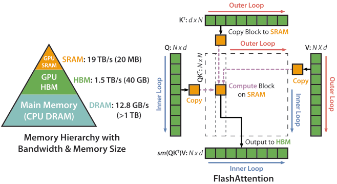
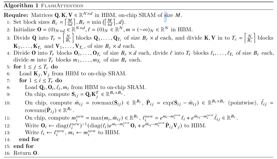
Flash Attention

Flash Attention^[11] reduces the frequency of visiting HBM and use tiling computation on self-attention computation. It uses K/V tiling in the outer loop and Q in inner loop in Flash Attention 1, and uses K/V for the inner loop to reduce the frequent SRAM visit.

References

---

1. 1.Shoeybi, M., Patwary, M., Puri, R., LeGresley, P., Casper, J., & Catanzaro, B. (2019). Megatron-lm: Training multi-billion parameter language models using model parallelism. arXiv preprint arXiv:1909.08053. ↩
2. 2.Narayanan, Deepak, et al. "Efficient large-scale language model training on gpu clusters using megatron-lm." Proceedings of the International Conference for High Performance Computing, Networking, Storage and Analysis. 2021. ↩
3. 3.Korthikanti, Vijay Anand, et al. "Reducing activation recomputation in large transformer models." Proceedings of Machine Learning and Systems 5 (2023): 341-353 ↩
4. 4.Rajbhandari, Samyam, Jeff Rasley, Olatunji Ruwase, and Yuxiong He. "Zero: Memory optimizations toward training trillion parameter models." In SC20: International Conference for High Performance Computing, Networking, Storage and Analysis, pp. 1-16. IEEE, 2020. ↩
5. 5.Huang, Yanping, et al. "GPipe: Easy Scaling with Micro-Batch Pipel ine Parallelism." Computer Vision and Pattern Recognition (2019). ↩
6. 6.Harlap, Aaron, et al. "Pipedream: Fast and efficient pipeline parallel dnn training." arXiv preprint arXiv:1806.03377 (2018). ↩
7. 7.Narayanan, Deepak, et al. "Memory-efficient pipeline-parallel dnn training." International Conference on Machine Learning. PMLR, 2021. ↩
8. 8.Zhao, Yanli, et al. "Pytorch fsdp: experiences on scaling fully sharded data parallel." arXiv preprint arXiv:2304.11277 (2023). ↩
9. 9.NVIDIA. Train with mixed Precision ↩
10. 10.Micikevicius, Paulius, et al. "Mixed precision training." arXiv preprint arXiv:1710.03740 (2017). ↩
11. 11.Dao, T., et al. "Fast and memory-efficient exact attention with io-awareness, 2022." URL https://arxiv. org/abs/2205.14135. ↩