Background: Conventional maximum likelihood approaches for sequence generation with teacher forcing algorithms are inherently prone to exposure bias at the inference stage due to the training-testing discrepancy—the generator produces a sequence iteratively conditioned on its previously predicted ones that may be never observed during training—leading to accumulative mismatch with the increment of generated sequences. In other words, the model is only trained on demonstrated behaviors (real data samples) but not free-running mode.
Generative Adversarial Networks (GANs) hold the promise of mitigating such issues for generating discrete sequences, such as language modeling, speech/music generation, etc.

GANs have demonstrated the compelling performance in generating real-valued data such as pixel-based images but have fallen short of discrete data generation primarily resulting from the incapability of gradient propagation passing from the discriminator (denoted as $\mathcal{D}$) to the generator (denoted as $\mathcal{G}$) in the original (image) GAN framework, which is incurred by the non-differential sampling/argmax operation in between.

Existing solutions to discrete sequence generation using GANs could be mainly sorted into different groups by resorting to:

Reinforcement Learning (RL): modeling the sequence generation procedure as a sequential decision-making process ^[1]^[6]^[7]^[8]; typically yielding high-variance but unbiased gradient estimates.
RL-free: utilizing soft-argmax operator^[2], Gumbel-softmax trick^[9], or continuous relaxation^[16] to provide the continuous approximation of the discrete distribution on the sequences; yielding low variance but biased estimation.

Summary

	Policy Gradient	Gumbel-softmax	Soft-argmax	Dense Reward	Internal Feature	Pretraining	$\mathcal{G}$	$\mathcal{D}$
SeqGAN (AAAI’17)	✔	✘	✘	✘	✘	✔	LSTM	CNN
TextGAN (ICML’17)	✘	✘	✔	✘	✔	✔	LSTM	CNN
MaliGAN (MILA)	✔	✘	✘	✘	✘	✔	LSTM	CNN
RankGAN (NIPS’17)	✔	✘	✔	✘	✘	✔	LSTM	CNN
LeakGAN (AAAI’18)	✔	✘	✔	✘	✔	✔	LSTM	CNN
GSGAN	✘	✔	✔	-	✘	-	LSTM	LSTM
FMGAN (NeurIPS’18)	✘	✘	✔	✘	✔	✔	LSTM	CNN
SentiGAN (IJCAI’18)	✔	✘	✘	✘	✘	✔	LSTM	CNN
MaskGAN (ICLR’18)	✔	✘	✘	✔	✘	✔	LSTM (seq2seq)	LSTM (seq2seq)
RelGAN (ICLR’19)	✘	✔	✔	✘	✘	✔	SAN	CNN
ScratchGAN (NeurIPS’19)	✔	✘	✘	✔	✘	✘	LSTM	LSTM
JSDGAN (AISTATS’19)	✘	✘	✘	✘	✘	✔ / ✘	N/A	✘
CatGAN (AAAI’20)	✘	✔	✔	✘	✘	✔	SAN	CNN
SALGAN (ICLR’20)	✔	✘	✘	✘	✘	✔	LSTM	CNN
ColdGAN (NeurIPS’20)	✔	✘	✔	✘	✘	✔	T5 / BART	N/A

SeqGAN (AAAI’17)

Problems

There exist limitations in discrete sequence generation using GANs, such as:

The discrete output of the generator $\mathcal{G}$;
$\mathcal{D}$ can only assess the complete sequence, while it is non-trivial to balance the current score and future one for partially generated sequence once the entire sequence has been generated.

Approach

SeqGAN^[1] bypasses the generator differentiation problem by directly performing a policy gradient update, which adopts the judgments of $\mathcal{D}$ on the complete generated sequences as reward signals using Monte Carlo (MC) search.

SeqGAN considers the sequence generation as a sequential decision-making process with a stochastic parameterized policy, in which the generator $\mathcal{G}$ is treated as the actor/agent of RL, the state is previously generated tokens so far and the action is the next token to be generated.

Image source: ^[1]

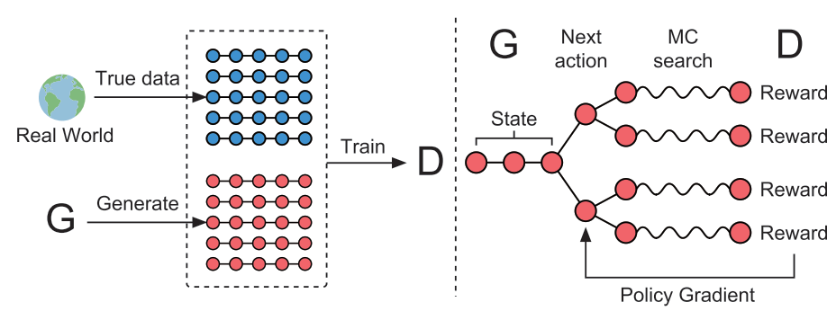
Definition

Given a dataset of real-word structured sequences, train a $\theta$-parameterized generative model $G_\theta$ to produce a sequence $Y_{1:T} = (y_1, \cdots, y_t, \cdots, y_T), y_t \in \mathcal{Y}$ , where $\mathcal{Y}$ is the vocabulary of candidate tokens. The policy $G_\theta(y_t \vert Y_{1: t-1})$ is stochastic: at the $t$-th timestep, the state $s$ is the current partially predicted sequences $(y_1, \cdots, y_{t-1})$ , and the action $a$ is the next token $y_t$ to be selected.

The discriminator $D_\phi$ parameterized by $\phi$ predicts how likely the sampled sequence $Y_{1:T}$ is from real data, providing the guidance (reward) to update the policy $G_\theta$ .

Policy Gradient with MC Search

Let $Q_{D_\phi}^{G_\theta} (s, a)$ be the action-value function of a sequence, i.e., the expected accumulative reward starting from the state $s$ taking action $a$ with policy $G_\theta$ ; $R_T$ be the reward for a complete sequence. The objective of $G_\theta(y_t \vert Y_{1:t-1})$ is to generate a sequence from the start state $s_0$ to maxmize its expected reward at the end of the episode:

$J(\theta) = \mathbb{E} [R_T \vert s_0, \theta] = \sum_{y_1 \in \mathcal{Y}} G_\theta (y_1 \vert s_0) \cdot Q_{D_\phi}^{G_\theta} (s_0, y_1).$

SeqGAN adopts the estimated probability of being real by $D_\phi (Y_{1:T}^n)$ as the reward, but $D$ can only provides the reward for a finished sequence. Thus, in order to evaluate the action-value for an intermediate state, Monte Carlo (MC) search with a roll-out policy $G_\beta$ is applied to sample the unknown last $T-t$ tokens. Let an $N$-time Monte Carlo search be $\{ Y_{1:T}, \cdots, Y_{1:T}^N \} = \textrm{MC}^{G_\beta}(Y_{1:T}; N)$ , where $Y_{1:t}^n = (y_1, \dots, y_t)$ and $Y_{t+1:T}^n$ is sampled based on the roll-out policy $G_\beta$ and the current state.

It runs the roll-out policy starting from current state till the end of the sequence for $N$ times to get a batch of output samples. Thus,

$\begin{align} \label{eq1}\tag{1} Q_{D_\phi}^{G_\theta} (s=Y_{1:t-1}, a=y_t) = \left\{ \begin{array}{ll} \frac{1}{N}\sum_{n=1}^N D_\phi(Y_{1:T}^n) & \textrm{for }t<T \\ D_\phi (Y_{1:t}) & \textrm{for }t=T \end{array} \right\}, \end{align}$

where $\quad Y_{1:T}^n \in \textrm{MC}^{G_\beta} (Y_{1:t}; N)$ . The intermediate reward is iteratively defined as the next-state value starting from the state $s^\prime = Y_{1:t}$ and rolling out to the end.

The $D_\phi$ is trained as follows:

$\begin{align} \label{eq2} \tag{2} \min_\phi - \mathbb{E}_{Y \sim p_\textrm{data}} [\log D_\phi (Y)] - \mathbb{E}_{Y \sim G_\theta} [\log (1-D_\phi (Y))]]. \end{align}$

The gradient of objective function $J(\theta)$ w.r.t. policy’s parameter $\theta$ is:

$\begin{align} \nabla_\theta J(\theta) &{}= \sum_{t=1}^T \mathbb{E}_{Y_{1:t-1} \sim G_\theta} \big[\sum_{y_t \in \mathcal{Y}} \nabla_\theta G_\theta (y_t \vert Y_{1:t-1}) \cdot Q_{D_\phi}^{G_\theta} (Y_{1:t-1}, y_t) \big] \\ &{}\simeq \sum_{t=1}^T \sum_{y_t \in \mathcal{Y}} \nabla_\theta G_\theta (y_t \vert Y_{1:t-1}) \cdot Q_{D_\phi}^{G_\theta} (Y_{1:t-1}, y_t) \\ &{}= \sum_{t=1}^T \sum_{y_t \in \mathcal{Y}} G_\theta (y_t \vert Y_{1:t-1}) \nabla_\theta \log G_\theta (y_t \vert Y_{1:t-1}) \cdot Q_{D_\phi}^{G_\theta} (Y_{1:t-1}, y_t) \\ &{}= \sum_{t=1}^T \mathbb{E}_{y_t \sim G_\theta (y_t \vert Y_{1:t-1})} \big[ \nabla_\theta \log G_\theta (y_t \vert Y_{1:t-1}) \cdot Q_{D_\phi}^{G_\theta} (Y_{1:t-1}, y_t) \big], \end{align}$

where $Y_{1:t-1}$ is the obvserved intermediate state sampled from $G_\theta$ .

Training Algorithm

Require: generator policy $G_\theta$ ; roll-out policy $G_\beta$ ; discriminator $D_\phi$ ; a sequence dataset $\mathcal{S}=\{ X_{1:T} \}$ ; learning rate $\alpha$

Initialize $G_\theta$ , $D_\phi$ with random weights $\theta$, $\phi$
Pretrain $G_\theta$ using MLE on $\mathcal{S}$
$\beta \leftarrow \theta$
Generate negative samples using $G_\theta$ for training $D_\phi$
Pretrain $D_\phi$ via minimizing the cross entropy
repeat
- for g-steps do
  1. Generate a sequence
    1. for $t$ in $1:T$ do
      - compute $Q(a=y_t; s=Y_{1:t-1})$ using Eq.(\ref{eq1})
  2. Update generator parameters with policy gradient: $\theta \leftarrow \theta + \alpha \nabla_\theta J(\theta)$
- for d-steps do
  - Use current $G_\theta$ to generate negative (synthetic) examples and combine with sampled positive (real) examples $\mathcal{S}$
  - Train discriminator $D_\phi$ for $k$ epochs using Eq.(\ref{eq2})
- $\beta \leftarrow \theta$
until SeqGAN converges

Model Architecture

Generator

$G_\theta$: LSTM actor.

$\begin{align} \mathbf{h}_t &{}= \textrm{LSTM}(\mathbf{h}_{t-1}, \mathbf{x}_t), \\ p(y_t \vert x_1, \cdots, x_t) &{}= \textrm{softmax} (\mathbf{c} + \mathbf{Vh}_t), \end{align}$

where $\mathbf{h}_{t-1}$ represents the $t$-th hidden state of LSTMs, $\mathbf{x}_t$ denotes the input embedding at the time step $t$.

Discriminator

$D_\phi$: CNN critic.
The input word embeddings are:

$\varepsilon = \mathbf{x}_1 \oplus \mathbf{x}_2 \oplus \cdots \oplus \mathbf{x}_T,$

where $\mathbf{x}_t \in \mathbb{R}^k$ represents the $k$ dimensional embedding, $\oplus$ is the vertical concatenation operator to build the matrix $\varepsilon_{1:T} \in \mathbb{R}^{T \times k}$. Then a kernel $\mathbf{w} \in \mathbb{R}^{n \times k}$ applies a convolutional operation to extract $n$-gram features:

$c_i = \rho (\mathbf{w} \otimes \varepsilon_{i:i+n-1} + b),$

where $\otimes$ operator is the summation of elementwise product, $b$ is a bias term, $\rho$ is a non-linear function. Then concatenate the output of multi-channel convolutions with various kernel sizes followed by a max-over-time-pooling:

$\begin{align} \mathbf{c} &{}= [c_1, \cdots, c_{T-l+1}], \\ \tilde{c} &{}= \max \{ \mathbf{c} \}. \end{align}$

Then apply a highway architecture before the final dense layer:

$\begin{align} \mathbf{\tau} &{}= \sigma (\mathbf{W}_T \cdot \tilde{\mathbf{c}} + \mathbf{b}_T), \\ \tilde{\mathbf{C}} &{}= \pmb{\tau} \cdot H(\tilde{\mathbf{c}}, \mathbf{W}_H) + (1-\pmb{\tau}) \cdot \tilde{\mathbf{c}}, \end{align}$

where $\mathbf{W}_T$ , $\mathbf{b}_T$ , $\mathbf{W}_H$ are highway layer weights, $H$ denotes an affine transform with non-linearity, $\pmb{\tau}$ represents the transform gate.

Finally, apply a sigmoid function to get the probability of being real given the input sequences:

$\hat{y} = \sigma (\mathbf{W}_o \cdot \tilde{\mathbf{C}} + \mathbf{b}_o),$

where $\mathbf{W}_o$ and $\mathbf{b}_o$ are the weight and bias respectively.

TextGAN (ICML’17)

Problems

Two fundamental problems of the GAN framework limit their usage in practice:

Mode collapse: $G$ tends to produce a single observation for multiple latent representations.^[3]
Vanishing gradient: $G$’s contribution to the learning signal is insubstantial when $D$ is close to its local optimum.^[4]

When $D$ is optimal, using standard GAN’s miminax objective is equivalent to minimizing the Jenson-Shannon Divergence (JSD)^[4] between the real data distribution $p_x(\cdot)$ and the synthetic data distribution $p_{\tilde{x}}(\cdot) \triangleq p\big( (G(z) )\big)$ , where $z \sim p_z(\cdot)$ . However, the saddile-point solution of the object is intractable. Thus iteratively updating $D$ and $G$ is required.

However, standard GAN’s objective suffers from unstable weak learning signal when $D$ gets close to its local minimum resulting from the vanishing gradient problem, which comes from that JSD implied by the original GAN objective approaches to a constant when $p_x(\cdot)$ and $p_{\tilde{x}}(\cdot)$ share no support, thus minimizing JSD yields no learning signal. This problem also exists in the distance metric of Total Variance Distance (TVD) of energy-based GAN (EBGAN).

Approach

TextGAN^[2] leverages the kernel-based moment-matching scheme over a Reproducing Kernel Hilbert Space (RKHS) to force the empirical distributions of real and synthetic sentences to have matched moments in latent-feature space, which consequentially ameliorates the mode collapsing issues associated with standard GAN training.

Objective Function

Given a sentence corpus $\mathcal{S}$, TextGAN proposes the objective:

$\begin{align} \mathcal{L}_D &{}= \mathcal{L}_\textrm{GAN} - \lambda_r \mathcal{L}_\textrm{recon} + \lambda_m \mathcal{L}_{\textrm{MMD}^2}, \tag{3}\label{eq3}\\ \mathcal{L}_G &{}= \mathcal{L}_{\textrm{MMD}^2}, \tag{4}\label{eq4}\\ \mathcal{L}_\textrm{GAN} &{}= \mathbb{E}_{s \sim \mathcal{S}}\log D(s) + \mathbb{E}_{z \sim p_z} \log [1- D(G(z))],\\ \mathcal{L}_\textrm{recon} &{}= \Vert \hat{z} - z \Vert^2, \end{align}$

where $\mathcal{L}_\textrm{recon}$ is the Euclidean distance between the reconstructed latent code $\hat{z}$ and the original code $z$ drawn from prior distribution $p_z(\cdot)$ ; $\mathcal{L}_{\textrm{MMD}^2}$ represents the Maximum Mean Discrepany (MMD) between the emprical distribution of sentence embeddings $\tilde{\mathbf{f}}$ and $\mathbf{f}$ for synthetic and real data respectively.

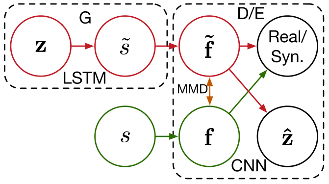
$\mathcal{L}(G)$ attempts to adjust to force the synthetic sentences’ features $\tilde{\mathbf{f}}$ to match the real sentence features $\mathbf{f}$ encoded by $D(\cdot)$, by matching the empirical distributions of $\tilde{\mathbf{f}}$ and $\mathbf{f}$ with a kernel discrepancy metric, MMD.

Analysis

In Eq.(\ref{eq3}), the reconstruction and MMD loss in $D$ serve as the regularizer to the binary classification loss in that $D$ features tend to be more spread out in the feature space.

Thus, $D(\cdot)$ attempts to select informative sentence features, whereas $G(\cdot)$ aims to match these features. Hyperparameters $\lambda_r$ and $\lambda_m$ act as the trade-off.

The original GAN objective is prone to mode collapsing especially when applying $\log D$ alternative for the generator loss, i.e., replacing the second term of Eq.(\ref{eq3}) with $-\mathbb{E}_{z\sim p_z} \log[D(G(z))]$ . If so, fake samples are more severely penalized than less diverse samples, thus grossly underestimating the variance of latent features^[3].

The $G$’s loss in Eq.(\ref{eq4}) forces $G$ to produce highly diverse sentences to match the variations of real data by latent moment matching, thus alleviating the mode-collapsing problem.

Feature Matching via MMD

MMD measures the mean squared difference between two sets of samples $\mathcal{X}$ andq $\mathcal{Y}$ over a RKHD $\mathcal{H}$ with kernel function $k(\cdot): \mathbb{R}^d \times \mathbb{R}^d \mapsto \mathbb{R}$, where $\mathcal{X}= \{ x_i \}_{i=1:N_x}, x_i \in \mathbb{R}^d$ , $\mathcal{Y}= \{ y_i \}_{i=1:N_y}, y_i \in \mathbb{R}^d$ . The kernel can be written as an inner product over $\mathcal{H}$: $k(x, x^\prime) = \langle k(x, \cdot), k(x^\prime, \cdot) \rangle_\mathcal{H}$ , and $\phi(x) \triangleq k(x, \cdot) \in \mathcal{H}$ denotes the feature mapping. Fomally the MMD between $\mathcal{X}$ and $\mathcal{Y}$ is given by:

$\begin{align} \mathcal{L}_{\text{MMD}^2} &{}= \| \mathbb{E}_{x \sim \mathcal{X}} \phi (x) - \mathbb{E}_{y \sim \mathcal{Y}} \phi(y) \|_\mathcal{H}^2 \\ &{}= \mathbb{E}_{x \sim \mathcal{X}} \mathbb{E}_{x^\prime \sim \mathcal{X}} [k(x, x^\prime)] + \mathbb{E}_{y \sim \mathcal{Y}} \mathbb{E}_{y^\prime \sim \mathcal{Y}}[k(y, y^\prime)] - 2 \mathbb{E}_{x \sim \mathcal{X}}\mathbb{E}_{y \sim \mathcal{Y}} [k(x,y)] \end{align}$

Here TextGANs adopt a gaussian (rbf) kernel $k(x,y)=\exp\big( - \frac{|x-y|^2}{2 \sigma} \big)$ with brandwidth $\sigma$.

Model Architecture

$G$: LSTM generator.
$D$: CNN discriminator.

MaliGAN (MILA)

Problems

Instability of GAN training: When optimizing $G$ USING $D$’s output as a reward via RL, the policy $G$ has difficulties to get positive and stable reward signals from $D$ even with careful pretraining.

When applying the GAN framework to discrete data, the discontinuity prohibits the update of the generator parameters via standard back-propagation. One way is to employ an RL strategy that directly uses the generator’s output, $D(\cdot)$, or $\log D(\cdot)$ as a reward.

Thus the objective for $G$ is to optimize:

$\begin{align} \mathcal{L}_\textrm{GAN} (\theta) &{}= - \mathbb{E}_{\mathbf{x} \sim p_\theta} [\log D(\mathbf{x})] \\ &{}\approx -\frac{1}{n} \sum_{i=1}^n \log D(\mathbf{x}_i), \quad \mathbf{x}_i \sim p_\theta. \end{align}$

Define the normalized probability distribution $q^\prime (\mathbf{x}) = \frac{1}{Z(D)}D(\mathbf{x})^{1/\tau}$ in some bounded region to guarantee the integrability ($D$ is an approxmation to $\frac{p_d}{p+p_d}$ if well trained) and also put a maximum-entropy regularizer $\mathbb{H}(p_\theta)$ to encourage diversity, yielding the regularized loss:

$\begin{align} \mathcal{L}_\textrm{GAN} (\theta) &{}= - \mathbb{E}_{\mathbf{x} \sim p_\theta} [\log D(\mathbf{x})] - \tau \mathbb{H}(p_\theta)\\ &{}= \tau \mathbb{KL}(p_\theta \| q^\prime) + c(D), \end{align}$

where $c(D)$ is a constant only depending on $D$. Hence, optimizing the original GAN is equivalent to minimizing the KL-divergence $\mathbb{KL}(p_\theta \| q^\prime)$ . However, since initially $p$ generates sentences with bad quality, it has little chance of generating good sequences to get a positive reward. Though with dedicated pre-training and variance reduction mechanisms, RL based on the moving reward signals still shows the unstable training and does not work on large scale datasets.

Approach

Maximum-Likelihood Augmented Discrete GAN (MaliGAN)^[7] utilizes the information of $D$ as an additional source of training signals on top of the maximum-likelihood objective, significantly reducing the variance during training.

Basic MaliGAN

MaliGAN keeps a delayed copy $p^\prime(\mathbf{x})$ of $G$ who is less often optimized. We know that the optimal $D$ is: $D(\mathbf{x})=\frac{p_d}{p_d + p^\prime}$ ; so we have $p_d=\frac{D}{1-D}p^\prime$ . Thus MaliGAN sets the target distribution $q$ for maximum likelihood training to be $\frac{D}{1-D}p^\prime$.

Let $r_D(\mathbf{x}) = \frac{D(\mathbf{x})}{1-D(\mathbf{x})}$ , we define the augmented target distribution as:

$q(\mathbf{x}) = \frac{1}{Z(\theta^\prime)} \frac{D(\mathbf{x})}{1-D(\mathbf{x})} p^\prime (\mathbf{x}) = \frac{1}{Z(\theta^\prime)} r_D(\mathbf{x}) p^\prime (\mathbf{x}).$

Regarding $q$ as a fixed probablity distribution, the target is to optimize:

$\mathcal{L}_G(\theta) = \mathbb{KL} (q(\mathbf{x}) \| p_\theta (\mathbf{x})).$

This objective has an attractive prob=perty that $q$ is a “fixed” distribution during training, i.e., if $D$ is sufficiently trained, then $q$ is always approximately the data generating distribution $q_d$ .
Defining the gradient as $\nabla \mathcal{L}_G = \mathbb{E}_q [\nabla_\theta \log p_\theta (\mathbf{x})]$ , we have:

$\begin{align} \nabla \mathcal{L}_G &{}= \mathbb{E}_{p^\prime} [\frac{q(\mathbf{x})}{p^\prime(\mathbf{x})} \nabla_\theta (\mathbf{x})] \\ &{}= \frac{1}{Z} \mathbb{E}_{p_\theta} [r_D (\mathbf{x})\nabla_\theta \log p_\theta (\mathbf{x})] , \end{align}$

where we assume that $p^\prime = p_\theta$ and the delayed generator is only one step behind the current update in the experiments.

Then $G$ is optimized as:

$\nabla \mathcal{L}_G (\theta) \approx \sum_{i=1}^m (\frac{r_D(\mathbf{x}_i)}{\sum_i r_D(\mathbf{x}_i)} - b) \nabla \log p_\theta (\mathbf{x}_i),$

where $b$ is the baseline to reduce variance. In practice, $b$ increases very slowly from 0 to 1 (as $D$).

Training

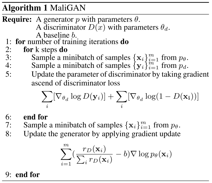
MaliGAN with Variance Reduction

Mixed MLE-Mali Training

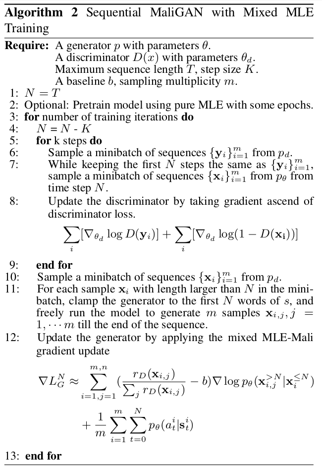
To alleviate the accumulated variance for long sequence generation, MaliGAN clamps the input using the training data for $N$ time steps< and switch to the free-running mode for the remaining $T-N$ time steps. During training, $N$ slowly moves from $T$ towards 0.

Thus,

$\begin{align} \nabla \mathcal{L}_G &{}= \mathbb{E}_q [\nabla \log p_\theta (\mathbf{x})]\\ &{}= \mathbb{E}_{p_d} [\nabla \log p_\theta (\mathbf{x}_{\leq N})] + \mathbb{E}_q [\nabla \log p_\theta (\mathbf{x}_{>N} \vert \mathbf{x}_{\leq N})] \\ &{}= \mathbb{E}_{p_d} [\nabla \log p_\theta (x_0, x_1, \cdots, x_T)] + \frac{1}{Z} \mathbb{E}_{p_\theta} [\sum_{t=N+1}^L r_D (\mathbf{x} \nabla \log p_\theta (a_t \vert \mathbf{s}_t))] \end{align}$

For each sample $\mathbf{x}_i$ from the real data batch, if it has length larger than $N$, we fix the first $N$ words of $\mathbf{x}_i$ , then sample $n$ times from $G$ till the end of the sequence and get $n$ samples $\{ \mathbf{x}_{i,j} \}_{j=1}^n$ . Then for each mini-batch with $0 \leq N \leq T$:

$\begin{align} \nabla \mathcal{L}_G^N \approx \sum_{i=1,j=1}^{m,n} \big(\frac{r_D(\mathbf{x}_{i,j})}{\sum_j r_D (\mathbf{x}_{i,j})} -b \big) \nabla \log p_\theta (\mathbf{x}_{>N} \vert \mathbf{x}_{\leq N}) + \frac{1}{m} \sum_{i=1}^m \sum_{t=0}^N p_\theta (a_t^i \vert \mathbf{s}_t^i) \end{align}$

Training

GSGAN (2016)

Problems

In the standard GAN framework, samples from a distribution on discrete objects such as multinomial are not differentiable w.r.t. the distribution parameters.

Gumbel-softmax Distribution

GSGAN^[9] uses the Gumbel-softmax distribution parameterized in terms of the softmax function to avoid the non-differential problem in GAN.

The softmax function can be used to parameterize a multinomial distribution on a one-hot-encoding $d$-dimensional vector $\mathbf{y}$ in terms of a continuous $d$-dimensional vector $\mathbf{h}$. Let $\mathbf{p}$ be a $d$-dimensional vector of probabilities specifying the multinomial distribution on $\mathbf{y}$ with $p_i = p(y_i=1), i=1,\cdots,d$ .

Then

$\mathbf{p} = \textrm{softmax}(\mathbf{h}),$

where $[\textrm{softmax}(\mathbf{h})]_i = \frac{\exp(\mathbf{h}_i)}{\sum_{j=1}^K \exp (\mathbf{h}_j)}, \textrm{for }i=1,\cdots,d$

Sampling $\mathbf{y}$ accoridng to the previous multinomial distribution with probability vector is the same as sampling $\mathbf{y}$ according to

$\mathbf{y}= \textrm{one_hot}(\arg\max_i (h_i + g_i)),$

where $g_i$ are independent and follow a Gumbel distribution with zero lcoation and unit scale. The sampled result has gradient zero w.r.t. $\mathbf{h}$ because the $\textrm{one_hot}(\arg\max(\cdot))$ is not differentiable. Thus, GSGAN propose to approximate with a differentiable function based on the soft-max transformtion:

$\mathbf{y} = \textrm{softmax}(\frac{1}{\tau} (\mathbf{h}+\mathbf{g})),$

where $\tau$ is an inverse temperature parameter. When $\tau \rightarrow 0$, the samples have the same output as argmax versionl when $\tau \rightarrow \infty$, the samples are always the uniform probability vector. GAN on discrete data can be trained with this, starting with soem relatively large $\tau$ and then annealing it to zero during training.

RankGAN (NIPS’17)

Problems

GANs assume the output of $D$ to be a binary predicate indicating whether the given sequence is from real or fake data, which is too restrictive since the diversity and richness of the sentences are constrained by the degenerated distribution due to binary classification.

Approach

RankGAN^[8] replaces the original binary classifier discriminator with a ranking model by taking a softmax over the expected cosine distances from the generated sequences to the real data. It relaxes the training of binary discriminator to a learning-to-rank optimization problem, consisting of a generator $G_\theta$ and a ranker $R_\phi$ . Instead of performing binary classification, the ranker is trained to rank the machine-generated sequences lower than the human-generated sequences.

$G$ is to confuse the ranker $R$ so that synthetic samples are ranked higher than real samples, while $R$ is to rank the synthetic sample (denoted “G” in the figure) lower than human-written setences (denoted “H” in the figure). Thus, $G$ and $R$ play a minimax game:

$\min_\theta \max_\phi \mathcal{L}(G_\theta, R_\phi) = \mathbb{E}_{s \sim \mathcal{P}_h} [\log R_\phi (s \vert U, C^-)] + \mathbb{E}_{s \sim G_\theta} [\log (1-R_\phi (s \vert U, C^+))],$

where $\mathcal{P}_h$ denotes the read data from human-written sentences, $C^+， C^-$ are comparison set w.r.t. different input $s$: when $s$ is the real data, $C^-$ generated data pre-sampled from $G_\theta$ ; If $s$ is the synthetic data, $C^+$ is the human written data.

Rank Score

The relevance score of the input sequence $s$ given a reference $u$ is:

$\alpha (s \vert u) = \cos (y_s, y_u) = \frac{y_s \cdot y_u}{\Vert y_s \Vert \Vert y_u \Vert},$

where $y_u$ and $y_s$ are embedded feature vectors of the reference and input sequence, respectively.

Then the ranking score for a sequence $s$ is computed given a comparison set $\mathcal{S}$:

$P(s \vert u, \mathcal{C}) = \frac{\exp (\gamma \alpha(s\vert u))}{\sum_{s^\prime \in \mathcal{C}^\prime} \exp (\gamma \alpha(s^\prime \vert u)) },$

which is similar to Boltzmann exploration in RL. Lower $\gamma$ results in all setenecs to be nearly equiprobable (uniform), while higher $\gamma$ increases the biases towards the sentence with higher score. $\mathcal{C}^\prime = \mathcal{C} \cup \{ s \}$ denotes the set of input sentences to be ranked.

Training

Like SeqGAN, RankGAN employs Monte Carlo rollout methods to simulate the intermediate rewards when a sequence is incomplete. The expected future reward $V$ for partial sequences is computed by:

$V_{\theta, \phi} (s_{1:t-1}, U) = \mathbb{E}_{s_r \sim G_\theta} [R_\phi (s_r \vert U, \mathcal{C}^+, s_{1:t-1})],$

where $s_r$ represents the complete setence sampled by rollout methods with given partial sequence $s_{1:t-1}$ . Specifically, the beginning tokens $(w_0, w_1, \cdots, w_{t-1})$ are fixed and the rest tokens are consecutively sampled by $G_\theta$ unitl the last token $w_T$ is generated. It samples $n$ times and take the average ranking score to approximate the expected reward.

The gradient of $G$’s objective is:

$\nabla_\theta \mathcal{L} (s_0) = \mathbb{E}_{s_{1:T} \sim G_\theta} \big[ \sum_{t=1}^T \sum_{w_t \in V} \nabla_\theta \pi_\theta (w_t \vert s_{1:t-1}) V_{\theta, \phi}(s_{1:t}, U) \big].$

In practice, minimizing $\log R(\cdot)$ instead of maximizing $\log (1-R(\cdot))$ performs better to train the ranker $R$. Thus, maximize the ranking objective:

$\max_\phi \mathcal{L}(G_\theta, R_\phi) = \mathbb{E}_{s \sim \mathcal{P}_h} [\log R_\phi (s \vert U, C^-)] - \mathbb{E}_{s \sim G_\theta} [\log R_\phi (s \vert U, C^+)],$

In a sense, replacing binary predicates with (multi-sentence) ranking scores can relieve the gradient vanishing problem.^[8]

LeakGAN (AAAI’18)

Problems

Sparsity: GANs with policy gradient can only get a scalar guiding signal after generating the entire texts and lack intermediate information about text structure during the generation process, which grossly hinders the generation of long texts (>20 words).
Non-informativeness: the scalar guiding signal for a whole text is non-informative as it does not necessarily preserve the picture about the intermediate syntactic and semantics of the text that is being generated for $G$ to sufficiently learn.

Approach

Inspired by Hierarchical Reinforcement Learning (HRL), LeakGAN^[6] designs a hierarchical generator $G$, consisting of a high-level “MANAGER” module and a low-level “WORKER” module. In each step, “MANAGER” receives $D$’s high-level feature representation to form the guiding goal for the “WORKER” module, which is a leakage of information from $D$. Then the “WORKER” module firstly encodes the currently generated tokens and combines with the goal embedding to take the final action at the current state. As such, the guiding signals from $D$ is available not only at the end but during the generation process.

LeakGAN can implicitly learn sentence structures, such as punctuation, clause structure, and long suffix without any supervision^[6].

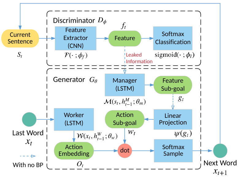
Feature Leakage from $D$

LeakGAN allows $D_\phi$ to provide additional information, i.e., feature $f_t$ of the current sequence $s_T$ to generate $G_\theta$ .

Typically, $D_\phi$ can be decomposed into a feature extractor $\mathcal{F}(\cdot ;\phi_f)$ and a final sigmoid classification layer with weight $\phi_l$ . Mathematically, given the input $s$, we have:

$D_\phi (s) = \sigma (\phi_l^\top \mathcal{F}(s;\phi_f)) = \sigma (\phi_l^\top f),$

where $f$ is the exxtracted features of CNN after max-over-time pooling.

In each time step $t$, “MANAGER” is an LSTM that takes the extracted feature vector $f_t$ and generates a goal vector $g_t$ , which is then fed into the “WORKER” module to guide the next word’s generation.

Generation

The “MANAGER” and “WORKER” of LSTMs are all zero-initialized. At each step, the “MANAGER” receives the leaked feature vector $f_t$ from the $D$ to produce the goal vector $g_t$ as:

$\begin{align} \hat{g}, h_t^M &{}= \mathcal{M} (f_t, h_{t-1}^M; \theta_m), \\ g_t &{}= \frac{\hat{g_t}}{\Vert g_t \Vert}, \end{align}$

where $\mathcal{M}(\cdot; \theta_m)$ denotes the LSTM of “MANAGER” with parameters $\theta_m$ and hidden vector $h_t^M$ .

The goal is a linear transformation $\psi$ with weight matrix $W_\psi$ with a summation over recent $c$ goals to produce a $k$-dimensional goal embedding $w_t$ as:

$w_t = \psi \big( \sum_{i=1}^c g_{t-i} \big) = W_\psi \big( \sum_{i=1}^c g_{t-i} \big).$

Then the “WORKER” takes the current word $x_t$ and combines the output with the goal embedding $w_t$ with a dot product before softmax:

$\begin{align} O_t, h_t^W &{}= \mathcal{W} (x_t, h_{t-1}^W; \theta_w), \\ G_\theta (\cdot \vert s_t) &{}= \textrm{softmax} (O_t \cdot w_t / \alpha), \end{align}$

where $\mathcal{W}(\cdot; \theta_w)$ denotes the LSTM of “WORKER”, $\alpha$ is the temperature to control the generation entropy.

Training of $G$

“MANAGER” is trained to predict advantageous directions in the discriminative feature space and the “WORKER” is intrinsically rewarded to follow such directions. The gradient of manager is defined as:

$\nabla_{\theta_m}^\textrm{adv} g_t = -Q_\mathcal{F} (s_t, g_t) \nabla_{\theta_m} \cos \big( f_{t+c}-f_t, g_t\big)$

where $Q_\mathcal{F} (s_t, g_t)= Q (s_t, g_t) = \mathbb{E} [r_t]$ is the expected reward under the current policy. $\cos(\cdot)$ measures the cosine similarity between the change of feature representation after $c$ step transitions, i.e., $f_{t+c}-f_t$ , and the goal vector $g_t$ . This loss functin is intuitively force the goal vector to match the transition inArrow the feature space while achieving high reward.

Meanwhile, the “WORKER” is trined to maximize the reaward using the REINFORCE algorithm:

$\nabla_{\theta_w} \mathbb{E}_{s_{t-1}\sim G} [\sum_{x_t} r_t^I \mathcal{W} (x_t \vert s_{t-1}; \theta_w)] = \mathbb{E}_{s_{t-1} \sim G, x_t \sim \mathcal{W}(x_t \vert s_{t-1})} [r_t^I \nabla_{\theta_w} \log \mathcal{W}(x_t \vert s_{t-1}; \theta_w)]$

where the intrinsit reward for “WORKER” $r_t^I$ is defined as:

$r_t^I = \frac{1}{c} \sum_{i=1}^c \cos \big( f_t - f_{t-i}, g_{t-i} \big).$

To be consistent, in pretraining stage, the gradient of “MANAGER” is:

$\nabla_{\theta_m}^\textrm{pre} g_t = - \nabla_{\theta_m} \cos(\hat{f}_{t+c} - \hat{f}_t, g_t)$

Interleaved training of MLE and GAN instead of full GAN training after pretraining. Blending these two training would help GAN get rid of some local minimum and alleviate mode collapse. Inserting MLE performs an implicit regularization on GAN to prevent it from going too far away from the MLE solution.

FM-GAN (NeurIPS’18)

Problems

TextGAN^[2] applied feature matching with MMD in the objective, which is difficult to train:

Choices of the bandwidth of the RBF kernel;
Kernel methods often suffer from poor scaling;
Empirically, TextGAN tends to generate short sentences.

Approach

Feature Mover GAN (FM-GAN)^[11] leverages earth-mover’s distance (EMD) in optimal transport (OT), which considers the problem of optimally transporting one set of data points to another. FM-GAN proposes feature-mover’s distance, a variant of EMD between the feature distribution of real and synthetic sentences. In this adversarial setting, $D$ aims to maximize the dissimilarity of the feature distributions based on the FMD, while the generator is trained to minimize the FMD by synthesizing more-realistic data.

See ^[11] for detailed formula of FMD.

MaskGAN (ICLR’18)

Problems

Training instability and mode dropping.

Approach

MaskGAN^[10] introduces an actor-critic conditional GAN that provides rewards at every time step. It fills in missing text conditioned on the surrounding context including text fill-in-the-blank or in-filling tasks, in which portions of the body of text are deleted or redacted. The goal of the model is to infill the missing portions of the text so that it is indistinguishable from the original data.

In-filling text: autoregressively output tokens that have thus far filled in as in standard language modeling while conditioned on the true known context.
If the entire body of the text is redacted, then this reduces to language modeling.

Architecture

Let $(x_t, y_t)$ denote pairs of input and target tokens; $\hat{x}_t$ is the filled-in token. Either real or fake $\hat{x}_t$ will be passed to $D$ during training.

MaskGAN uses seq2seq encoder-decoder architecture. For a discrete sequence $\mathbf{x}= (x_1, \cdots, x_T)$ , a binary mask is generated of the same length $\mathbf{m}=(m_1, \cdots, m_T)$ where $m_t \in \{ 0,1 \}$ determining whether to retain or mask.

The masked sequence $\mathbf{m}(\mathbf{x})$ is fed to the encoder (as below figure), and the decoder fills in missing tokens auto-regressively conditioned on both the masked input and what has filled-in upfront. The generator decomposes the distribution over the sequence into an ordered conditional sequence:

$G(x_t) \equiv P(\hat{x}_1, \cdots, \hat{x}_T \vert \mathbf{m(x)}) = \prod_{t=1}^T P(\hat{x}_t \vert \hat{x}_1, \cdots, \hat{x}_{t-1}, \mathbf{m(x)}).$

Generator architecture^[10]

The discriminator $D$ has the identical architecture to $G$ except the scalar output at each time step, computing the probability of each token $\tilde{x}_t$ being real given the true context of masked sequences $\mathbf{m(x)}$:

$D_\phi (\tilde{x}_t \vert \tilde{x}_{0:T}, \mathbf{m(x)}) = P(\tilde{x}_t = x_t^\textrm{real} \vert \tilde{x}_{0:T}, \mathbf{m(x)}).$

The logrithm of the $D$’s estimates are regarded as the reward:

$r_t \equiv \log D_\phi (\tilde{x}_t \vert \tilde{x}_{0:T}, \mathbf{m(x)}).$

The critic net is an additional head off the discriminator, estimating the value function in RL.

Training

MaskGAN employs policy gradient estimation for generator $G$:

$\begin{align} \nabla_\theta \mathbb{E}_G [R_t] &{}= (R_t - b_t) \nabla_\theta G_\theta (\hat{x}_t) \\ &{}= \mathbb{E}_{\hat{x}_t \sim G} \big[ \sum_{t=1}^T (R_t -b) \nabla_\theta \log G_\theta(\hat{x}_t) \big] \\ &{}= \mathbb{E}_{\hat{x}_t \sim G} \big[ \sum_{t=1}^T (\gamma^s r_s - b_t) \nabla_\theta \log G_\theta (\hat{x}_t) \big], \end{align}$

where $gamma$ is the discount vector, $b_t$ is the critic.

Finally, $D$ is updated with:

$\nabla_\phi \frac{1}{m} \sum_{i=1}^m \big[ \log D(x^{(i)}) + \log (1-D(G(z^{(i)}))) \big]$

Pretraining:

Trin LM using MLE for encoder/decoder.
Then pretrain the seq2seq model on the in-filling task using MLE. Select with holdout set.
Not include critic.

SentiGAN (IJCAI’18)

SentiGAN^[12] employs $k$ generators with $k$ sentiment labels and one multi-class ($k+1$) discriminator.

Let $S_t$ represent the partially generated sequence $S_t = \{ X_1, \cdots, X_t \}$ , where $X_t$ is a token generated at time $t$. It defines the penalty based loss function at step $t$ for $G$:

$\mathcal{L}(X) = G_i (X_{t+1} \vert S_t) \cdot V_D^G (S_t, X_{t+1}),$

where $V_D^G (S_t, X_{t+1})$ is generated by $D$.

The objective of $G$ is defined with MC search:

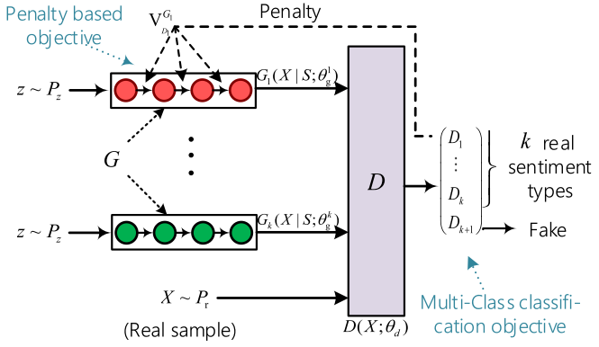
$\begin{align} J_G &= \mathbb{E}_{X \sim P_g} [\mathcal{L}(X)] \\ &= \sum_{t=0}^{t= \vert X \vert -1} G (X_{t+1} \vert S_t) \cdot V_D^G (S_t, X_{t+1}) \end{align}$

$D$ is a CNN-based multi-class discriminator, producing a ${k+1}$-dimensional probability vector. The score at $i$-th ($i \in {1,\cdots,k}$) index represents the probablity of being the $i$-th sentiment, the $(k+1)$-th index denote the probability to be synthetic.

Refer to ^[12] for details.

RelGAN (ICLR’19)

Problems

GANs suffer from mode collapse issue due to either a lack of expressive power in $G$ (not considering many more complex modes in the data distribution), or by a less informative guiding signal in $D$ (constrain the $G$’s update to within certain modes).

The LSTM-based generator might be the bottleneck of GANs with such experimental observations:

$D$’s loss value very quickly goes t near minimum after few iterations, which means $D$ may be more powerful than $G$ and can easily distinguish between real/fake samples;
Mode collapse may partly indicate the incapacity of $G$, as it may not be expressive enough to fit all modes of data distribution;
Existing GANs perform poorly at long sentence generation, and LSTM encodes all previous sequences into a fixed hidden vector, potentially limiting its ability to modeling long-distance dependency.

Approach

RelGAN^[13] employs a relational memory based generator; Gumbel-softmax trick; and multi-representations in $D$.

Relational Memory based $G$

As below figure, let each row of the memory $M_t$ denote a memory slot. Given input $x_t$ at time $t$ and $H$ heads, the memory is updated with self-attention mechanisms.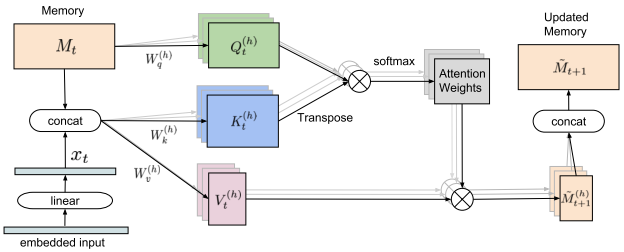

For each head, we have query $Q_t = M_t W_q$ , key $K_t = [M_t; x_t] W_k$ , and value $V_t = [M_t;x_t]W_v$ , where $[;]$ denotes row-wise concatenation. Thus, the updated memory $\tilde{M}_{t+1}$ :

$\begin{align} \tilde{M}_{t+1} &{}= [\tilde{M}_{t+1}^{(1)}L\cdots :\tilde{M}_{t+1}^{(H)}],\\ \tilde{M}_{t+1}^{(h)} &{}= \textrm{softmax}\big( d_k^{-1/2} M_t W_q ([M_t;x_t] W_k)^\top \big) [M_t;x_t] W_v, \end{align}$

where $d_k$ is the column dimension of $K_t$ , $[:]$ denotes column-wise concatenation.

Then the next memory $M_{t+1}$ is computed with skip-connections/MLP/gated operations.

Gumbel-Softmax Relaxation

The multinomial softmax can be parameterized as:

$y_{t+1} = \textrm{one_hot} (\arg\max_{1\leq i \leq V} (o_t^{(i)} + g_t^{(i)})),$

where $o_t^{(i)}$ denotes the $i$-th entry of $o_t$ and $g_t^{(i)}$ is from the $i.i.d.$ Gumbel distribution $g_t^{(i)} = -\log \big( -\log U_t^{(i)} \big)$ with $U_t^{(i)} \sim \textrm{uniform}(0,1)$ .

Further, the one-hot with argmax op can be approximated as:

$\hat{y}_{t+1} = \textrm{sofmtax} \big( \beta (o_t + g_t) \big),$

where the incerse temperature $\beta \in \mathbb{R}+$ is a tunable parameter. Large $\beta$ encourages exploration for better sample diversity while smaller one does more explitation for bettter sample quality.

Thus it has an exponential policy: $\beta_n = \beta_\max^{n/N}$ , where $\beta_\max$ denotes the maximum inverse temperature, $N$ is the maximum # of training iteration, $n$ denotes current iteration. The increase rate of inverse temperature is from exploitation phrase to exploration phrase.

Multiple Representaions in $D$

RelGAN applies multiple embedded representations for each input with each independently passed through CNN-based classifiers to get the score. Finally, take the average of different representations as the final guiding signal to update $G$. This resembles the use of multiple discriminators in image GANs but keeps a weight-sharing CNN-based classifier to curtail the computational cost.

Training

Loss function

RelGAN use the loss of Relativistic GAN (RSGAN), i.e., $f(a,b) = \log \sigma (a-b)$ for $a,b \in \mathbb{R}$.
Thus,

$\mathcal{L}_D = \frac{1}{S} \sum_{s=1}^S \mathbb{E}_{r_{1:T}\sim P_R; \hat{y}_{1:T}\sim P_\theta} \log \sigma \big( D(\tilde{X}_r^{(s)}) - D(\tilde{X}_y^{(s)}) \big).$

Intuitively, this loss is to directly estimate the average probability that real sentences are more realistic than generated sentences in terms of different embedded representations.

ScratchGAN (NeurIPS’19)

Problems

Having suffered from challenges with gradient estimation, optimization instability, and mode collapse, existing language GANs resorted to MLE pretraining followed by adversarial fine-tuning with restrictive fine-tuning epochs and a small learning rate.
This suggests that “the best-performing GANs tend to stay close to the solution given by MLE training”. Even with pre-training, it shows that discrete GANs do not improve over MLE training.

Learning Signals

The REINFORCE gradient estimator for $G$:

$\nabla_\theta \mathbb{E}_{p_\theta (\mathbf{x})} [R(\mathbf{x})] = \mathbb{E}_{p_\theta (\mathbf{x})}[R(\mathbf{x}) \nabla_\theta \log p_\theta (\mathbf{x}) ],$

where $R(\mathbf{x})$ is provided by $D(\cdot)$. When setting $R(\mathbf{x})=\frac{p^*(\mathbf{x})}{p_\theta(\mathbf{x})}$ , it recovers the MLE estimator:

$\mathbb{E}_{p_\theta (\mathbf{x})}[\frac{p^*(\mathbf{x})}{p_\theta(\mathbf{x})} \nabla_\theta \log p_\theta (\mathbf{x}) ] = \mathbb{E}_{p^*(\mathbf{x})}[\nabla_\theta \log p_\theta (\mathbf{x})] = \nabla_\theta\mathbb{E}_{p^*(\mathbf{x})}\log p_\theta (\mathbf{x}).$

The gradient updates of MLE can be seen as a special case of the REINFORCE updates in discrete GAN training, whereas the language GANs’ rewards are learned.

We postulate the learned rewards provide a smoother signal to $G$ than classical MLE loss: $D$ can learn to generalize and provide a meaningful signal over parts of the distribution uncovered by the training data. As the training progresses and the signal from $D$ improves, $G$ also explores other parts of the data space, providing a natural curriculum, whereas MLE training is only exposed to the expert demonstration (real data).

Approach

ScratchGAN^[14] combines existing techniques such as large batch sizes, dense rewards, and discriminator regularization to stabilize and improve the discrete GANs.

Dense Rewards

ScratchGAN emplolys a recurrent discriminator to provide rewards for each generated token. The discriminator learns to distinguish between sentence prefixees coming from real data and sampled sentence prefixes:

$\max_\phi \sum_{i=1}^T \mathbb{E}_{p^*(x_t \vert x_1, \cdots, x_{t-1})} [\log D_\phi (x_t \vert x_1, \cdots, x_{t-1})] + \sum_{t=1}^T \mathbb{E}_{p_\theta(x_t \vert x_1, \cdots, x_{t-1})} [1-\log D_\phi (x_t \vert x_1, \cdots, x_{t-1})].$

The recurrent $D$ is much cheaper than Monte Carlo Tree Search (MCTS) to score partial sentences.

FOr the geerated token $\hat{x}_t \sim p_\theta (x_t \vert x_1, \cdots, x_{t-1})$ , the reward at time step $t$ is scaled linearly with $D$’s output:

$r_t = 2 D_\phi (\hat{x}_t \vert x_1, \cdots, x_{t-1}) -1.$

The goal of $G$ at timestep $t$ is to maximize the sum of discounted future rewards using a discount factor $\gamma$:

$R_t = \sum_{s=t}^T \gamma^{s-t} r_s.$

Large Batch Size for Variance Reduction

$G$ is updated using MC estimates of policy gradients, where $N$ is the batch size:

$\nabla_\theta = \sum_{n=1}^N \sum_{t=1}^T (R_t^n - b_t) \nabla_\theta \log p_\theta (\hat{x}_t^n \vert \hat{x}_1^n , \cdots, \hat{x}_{t-1}^n ), \quad \hat{x}_t^n \sim p_\theta (\hat{x}_t^n \vert \hat{x}_1^n , \cdots ,\hat{x}_{t-1}^n )$

ScratchGAN uses a global moving-average of rewards as a baseline $b_t$ .

Training

$D$ and $G$ both use an embedding layer followed by one or more LSTM layers.
Discriminator regularization: layer normalization, dropout, L₂ weight decay.
Concatenating the fixed sinusoidal position matrices and word embeddings in $D$.

JSDGAN (AISTATS’19)

Background

MLE is equivalent to minimizing the KL divergence between the empirical data distribution and the model distribution, which tends to favor approximations of model distribtuion that overgeneralize the data distribtuion. Instead the reverse KL divergence favors under-generalization. JSD combines KL and reverse KL, which is symmetric.

GAN is regarded as a two-play minimax game with distinguishability game value function $V(G,D)$:

$\min_G \max_D V(G,D) = \mathbb{E}_{x \sim \tilde{p}_\textrm{data}(x)} \log D(x) + \mathbb{E}_{x \sim p_G (x)} \log (1-D(x)),$

where $\tilde{p}_\textrm{data}(x)$ denotes the empirical data distribution over training data $\mathcal{C}=\{ x_1, \cdots, x_N \}$ , and

$\tilde{p}_\textrm{data}(x) = \left\{ \begin{array}{ll} \frac{1}{N} & \textrm{if } x \in \mathcal{C} \\ 0 & \textrm{otherwise} \end{array} \right.$

GAN without Explicit $D$

^[15] claimed that optimal $D$ has a closed form solution, and approximation on $D$ with neural networks is unnecessary.
It directly optimizes the JSD divergence between the distribution between $G$ and real data without sampling from $G$, which implies an alternative minimax optimizatin procedure.

The optimal discriminator $D^*_G (x)$ is:

$D^*_G (x) = \left\{ \begin{array}{ll} \frac{\tilde{p}_\textrm{data}(x)}{\tilde{p}_\textrm{data}(x) + p_g(x)} & \textrm{if } x \in \mathcal{C} \\ 0 & \textrm{otherwise} \end{array} \right.$

The value function with optimal $D^*_G(x)$ becomes:

$\begin{align} V(G, D^*_G (x)) &= 2 \textrm{JSD} (\tilde{p}_\textrm{data}(x) \Vert p_G (x)) - \log 4 \\ &= \sum_{x \in \mathcal{C}} \tilde{p}_\textrm{data} \log [ \frac{\tilde{p}_\textrm{data}(x)}{\tilde{p}_\textrm{data}(x) + p_g(x)} ] + \sum_{x \in \mathcal{C}} p_G (x) [\log \frac{p_g(x)}{\tilde{p}_\textrm{data}(x) + p_g(x)} ] \end{align}$

This approach is only applicable when $p_G(x)$ has explicit representations.

CatGAN (AAAI’20)

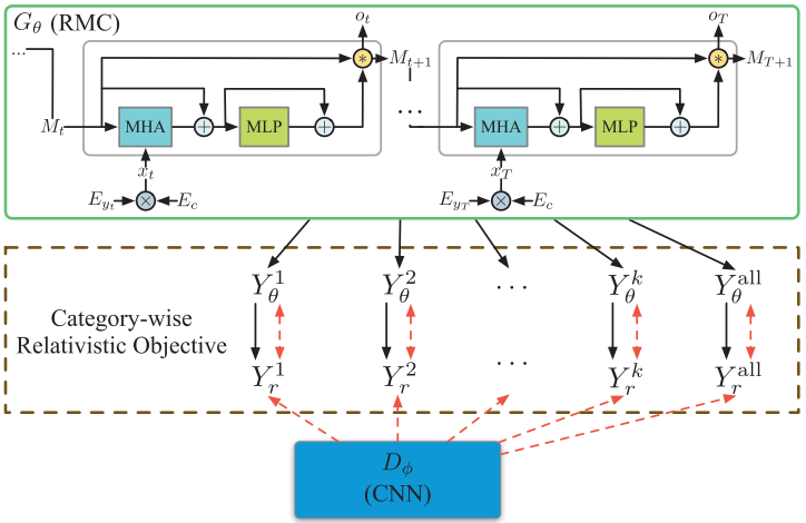
Category-aware GAN (CatGAN)^[18] employs such methods to generate sentences of different categories:

Gumbel-softmax relaxation (as ^[13])
SAN-based relational memory (as ^[13])
Category-wise relativistic objective.
Hierarchical evolutionary learning.

SALGAN (ICLR’20)

Problems

Reward spasity
Mode collapse

Comparative discriminaor

SALGAN^[17] employs a comparative discriminaor to pairwisely compare the text quality between a pair of samples: better($>$), worse ($<$), or indistinguishable ($\approx$). Given a training set with $n$ real samples and $n$ generated samples, the comparative discimination can construct $\binom{2n}{2}$ pairwise training examples.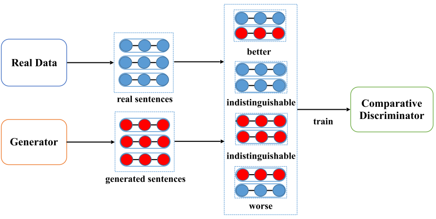

ColdGAN

ColdGAN^[19] adopts such methods on T5 (small) and BART:

Importance sampling
PPO Clip
Nucleus sampling

References

1.Yu, Lantao, et al. "Seqgan: Sequence generative adversarial nets with policy gradient." Thirty-first AAAI conference on artificial intelligence. (2017). ↩
2.Zhang, Yizhe, et al. "Adversarial feature matching for text generation." arXiv preprint arXiv:1706.03850 (2017). ↩
3.Metz, Luke, et al. "Unrolled generative adversarial networks." arXiv preprint arXiv:1611.02163 (2016). ↩
4.Arjovsky, Martin, and Léon Bottou. "Towards principled methods for training generative adversarial networks." arXiv preprint arXiv:1701.04862 (2017). ↩
5.Goodfellow, Ian, et al. "Generative adversarial nets." Advances in neural information processing systems (2014). ↩
6.Guo, Jiaxian, et al. "Long text generation via adversarial training with leaked information." Thirty-Second AAAI Conference on Artificial Intelligence (2018). ↩
7.Che, Tong, et al. "Maximum-likelihood augmented discrete generative adversarial networks." arXiv preprint arXiv:1702.07983 (2017). ↩
8.Lin, Kevin, et al. "Adversarial ranking for language generation." Advances in Neural Information Processing Systems (2017). ↩
9.Kusner, Matt J., and José Miguel Hernández-Lobato. "Gans for sequences of discrete elements with the gumbel-softmax distribution." arXiv preprint arXiv:1611.04051 (2016). ↩
10.Fedus, William, Ian Goodfellow, and Andrew M. Dai. "MaskGAN: Better text generation via filling in the _." ICLR (2018). ↩
11.Chen, Liqun, et al. "Adversarial text generation via feature-mover's distance." Advances in Neural Information Processing Systems (2018). ↩
12.Wang, Ke, and Xiaojun Wan. "SentiGAN: Generating Sentimental Texts via Mixture Adversarial Networks." IJCAI (2018). ↩
13.Nie, Weili, Nina Narodytska, and Ankit Patel. "Relgan: Relational generative adversarial networks for text generation." International conference on learning representations (2019). ↩
14.de Masson d'Autume, Cyprien, et al. "Training language gans from scratch." Advances in Neural Information Processing Systems (2019). ↩
15.Li, Zhongliang, et al. "Adversarial discrete sequence generation without explicit neuralnetworks as discriminators." The 22nd International Conference on Artificial Intelligence and Statistics (2019). ↩
16.Gulrajani, Ishaan, et al. "Improved training of wasserstein gans." Advances in Sneural information processing systems (2017). ↩
17.Zhou, Wangchunshu, et al. "Self-Adversarial Learning with Comparative Discrimination for Text Generation." arXiv preprint arXiv:2001.11691 (2020). ↩
18.Liu, Zhiyue, Jiahai Wang, and Zhiwei Liang. "CatGAN: Category-Aware Generative Adversarial Networks with Hierarchical Evolutionary Learning for Category Text Generation." AAAI. 2020. ↩
19.Scialom, Thomas, et al. "ColdGANs: Taming Language GANs with Cautious Sampling Strategies." arXiv preprint arXiv:2006.04643 (2020). ↩