A summary of image-to-text translation.
Neural Image Captioning (CVPR 2015)
As the first end-to-end neural model for image captioning tasks, Neural Image Captioning (NIC)[1] combines the pretrained convolutional neural networks (CNNs) for image classification with recurrent networks (RNNs) for sequence modeling.
Let $I$ denote the input image, be the $D$-dimensional word embedding matrices of vocabulary $V$, be the one-hot vector of $t$-th word.
Inference: sampling or beam search.
Show, Attend and Tell (ICML 2015)
The model receives a single raw image and generates a caption encoded as a sequence of $1$-of-$V$ encoded words.
where $V$ is the vocabulary size and $C$ is the caption length.
Encoder
- Encoder: employ CNNs (Oxford VGGnet) from lower convolutional layers (4-th convolutional layer before max-pooling. 14 x 14 x 512) to extract $L$ (14 x 14 =196) vectors for each image. $D$-dimensional (512) features corresponds to different part of the images.
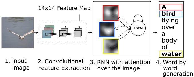
Decoder
- Decoder: LSTMwhere denotes affine transformation, , , , , are the input, forget, memory, output and hidden state of the LSTM, respectively.
The context vector is calculated as:
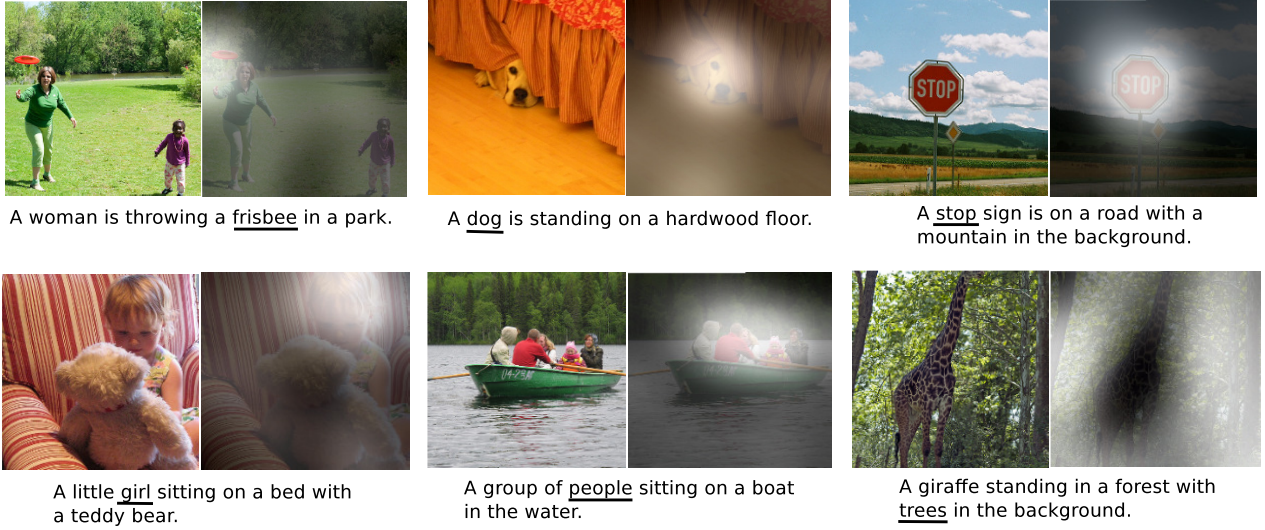
where represents the position weight, indicating as either the probability that location $i$ is the right place to focus on, or as relative importance to give to location $i$ in blending the ‘s together. “Where” the network looks next, i.e., , depends on the sequence of words that has already been generated, i.e., .
The initial memory state and hidden state of the LSTM are linear projected outputs of an average of annotation vectors :
- Output: use a deep output layer with LSTM state, context vector and the previous word:where and $\mathbb{E}$ are learnable parameters initialized randomly.
Attention
fatt has two alternatives:
- stochastic (hard) attention
- deterministic (soft) attention.
Stochastic Hard Attention
Let the location variable denote where the model to focus on when generating the $t$-th word. is an indicator one-hot variable where the $i$-th location to focus is set to 1. They assign a multinouli distribution parameterized by . This method requires sampling the attention location at each time $t$.
It is computed as:
The objective function $L$ is defined as a variational lower bound on the marginal log-likelihood of obsreving sequence of words $\mathbf{y}$ given image features $\mathbf{a}$. Let $W$ denote the parameters of the model.
By assuming , the location is calculated by sampling with Monte Carlo method.
A moveing average baseline is used to reduce the variance in the Monte Carlo estimator:
Finally, the entropy term is added:
where and are discounting factors.
This equation is equivalent to the REINFORCE learning, where the reward for selecting the attention is a real value proportional to the log-likelihood of the target sentence under the sampled attention rollouts.
Deterministic Soft Attention
Soft attention take the expectation of the context vector $\hat{\mathbf{z}}_t$ directly:
Deterministic soft attention can be treated as an approximation to the marginal likelihood over the attention locations.
The expectation can be treated as the first order Taylor approximation using a single forward prop.
Let , denote computed by setting the context vector $\hat{\mathbf{z}}$ value to . The normalized weighted geometric mean for the softmax $k$-th word prediction:
It show that the expectation of context vector .
Doubly Stochastic Attention
- Encourage
- Adopt a gating scalar $\beta$ from previsou hidden state at each time step $t$
- The model is trained end-to-end by minimizing the penalized negative log-likelihood:
Training
- Trained both attention variants using SGD with an adaptive learning rate. They found that RMSProp worked best on Flickr8k, whereas Adam performed better on Flickr30k/MS COCO dataset.
- Early stopping on BLEU score, dropout.
- MS COCO: < 3 days training on an NVIDIA Titan Black GPU.
- Vocabulary size V=10k.
- Problems: no public splits on Flickr30k and COCO datasets.
- Single model w/o an ensemble.
Semantic Attention (CVPR 2016)
Image captioning methods can be generally divided into two approaches: top-down and bottom-up.
- The top-down method starts from the image features and converts it into words end-to-end using RNNs. But it is hard to attend to fine details when describing the image.
- The bottom-up method is free to operate on any image resolution but lacks end-to-end formulation.
Architecture
Semantic Attention[4] extracts top-down and bottom-up features from an input image. Firstly, the global visual feature $\mathbf{v}$ is extracted from a classification CNN and a list of visual attributes or concepts that are detected using attribute detectors.
$\mathbf{v}$ is only used to initilize the input node .
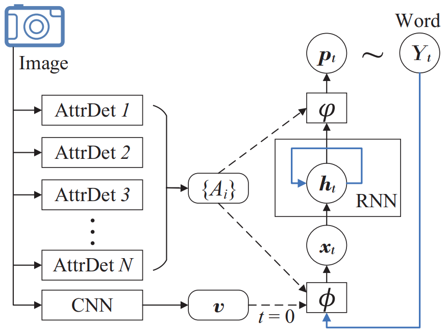
Input attention $\phi$
Both and correspond to an one-hot entry in dictionay $\mathcal{Y}$, denoting as and , respectively. Let with $d << \vert \mathcal{Y} \vert$, the relevance score assigned to each detected attribute based on its relevance between the previous predicted word :
where trainable parameters $\mathbf{U} \in \mathbb{R}^{d \times d}$
The attention score $\alpha$ measures the attention on different attributes. The weighted sum are added to the input space together with previous word:
where is the project matrix, $\mathbf{w}^{x,A} \in \mathbb{R}^d$ models the relative importance of visual attributes in each dimension of the word space.
Output attention $\varphi$
Similarly, the score for each attribute is measured w.r.t :
The sigmiod activation function $\sigma$ is applied as the output to hidden state in RNN to ensure the same nonlinear transform on compared feature vectors.
The distribution is generated by a linaer transform followed by a softmax normalization:
where $\mathbf{W}^{Y,h} \in \mathbf{R}^{d \times n}$ is the projection matrix and $\mathbf{w}^{Y,A} \in \mathbf{R}^n$ models the relative importance of visual attributes in each dimension of the RNN state space.
Model training
The loss function is defined as the NLL loss combined with regularization terms on attention scores and :
where and are attention score matrices with $(t,i)$-th entries of and . The regularization function $g$ is used to enfoce the completeness of attention paid to every attribute in as well as the sparsity of attention at any particular time step.
where the first term with $p>1$ penalizes excessive attention paid to any single attribute accumulated over the entire sentence, and the second term $0<q<1$ penalizes diverted attention to multiple attributes at any particular time.
SCA-CNN (CVPR 2017)
Motivation:
- low-layer filters detect low-level visual cues like edges and corners, while higher-level ones extract abstract semantic patterns like objects.
- CNN extractors output a hierarchy of visual abstractions, which is spatial, channel-wise, and multi-layer. Previous work only takes into account the spatial characteristics, regardless of the channel-wise and multi-layer information.
- SCA-CNN takes full advantage of such three characteristics of CNN features.
Spatial and Channel-wise Attention CNN
Spatial and Channel-wise Attention-based Convolutional Neural Network (SCA-CNN)[5] applies channel-wise attention and spatial attention at multiple layers.
At $l$-th layer, the spatial and channel-wise attention weights $\gamma^l$ are function of LSTM memory and input CNN features $\mathbf{V}^l$, where $d$ is the dimension of hidden state. SCA-CNN modulates using the spatial and channel attention weights $\gamma^l$ as follows:
where is the modulated feature, $\pmb{\Phi}(\cdot)$ is the spatial and channel-wise attention function, $f(\cdot)$ is a linear weighting function that modulates CNN features and attention weights.
The spatial attention weights $\alpha^l$ and channel-wise attention weights $\beta^l$ are learned separately:
where and represent spatial and channel-wise model respectively, having the cost of for spatial attention and $\mathcal{O}(C^lk)$ for channel-wise attention. $W$,$H$,$C$, $k$ represent the width, height, channel and mapping dimension.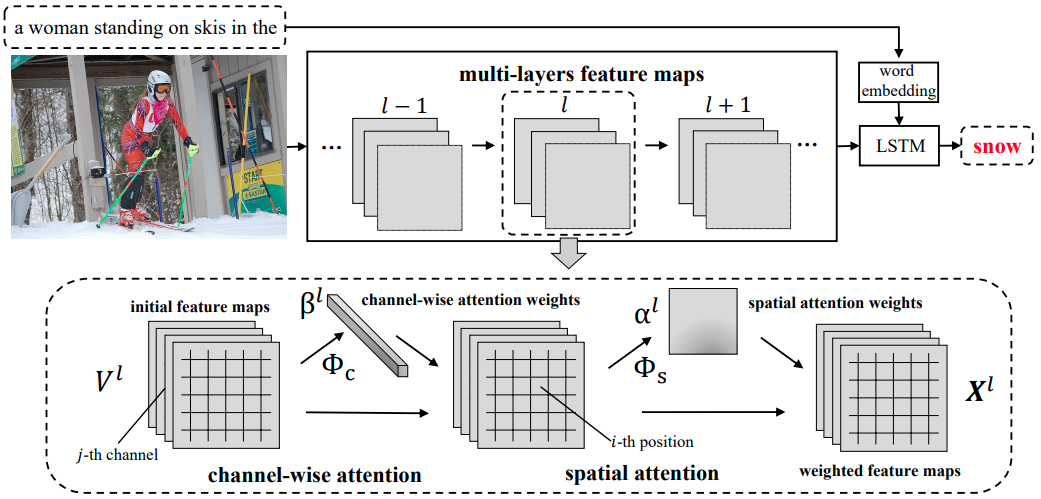
Spatial Attention
CNN features is flattened features along width and height, where , and $m=W \cdot H$. is considered as the visual feature of the $i$-th location. Given the previous hidden state , a single-layer fully-connected layer followed by a softmax is applied to generate attention distributions $\alpha$ over the image regions.
where , , are trainable matrices to obtain the same dimension $k$, $\oplus$ is the addition between a matrice and a vector, model biases .
Channel-wise Attention
Each CNN filter is a pattern detector on images, and each channel of a feature map in CNN is a response activation of the corresponding convolutional filter. Applying channel-wise attention mechanisms can be treated as selecting semantic attributes.
Firstly, CNN features $\mathbf{V}$ is reshaped to $\mathbf{U} = [\mathbf{u}_1, \mathbf{u}_2,\cdots, \mathbf{u}_C]$, where represents the $i$-th channel of the feature map $\mathbf{V}$, $C$ is the channel number. The mean-pooling for each channel is applied to obtain the channel feature $\mathbf{v}$:
where scalar is the mean of vector , which represents the $i$-th channel features.
The channel-wise attention model $\Phi_c$ can be defined as:
where are trainable parameters, $\otimes$ represents the outer product of vectors, biases .
Channel-Spatial
Apply channel-wise attention followed by feature map $\mathbf{X}$.
where is a channel-wise multiplication for feature map channels and corresponding channel weights.
Adaptive Attention (CVPR 2017)
Motivation:
- Most attention-based methods force visual attention to be active for each generated word. However, not all words have corresponding visual signals.
- Decoders require little to predict words like “the”/“of”. Besides, other words that may be predicted reliably just from the language model, e.g.,, “sign” after “behind a red stop” or “phone” following “talk on a cell”.
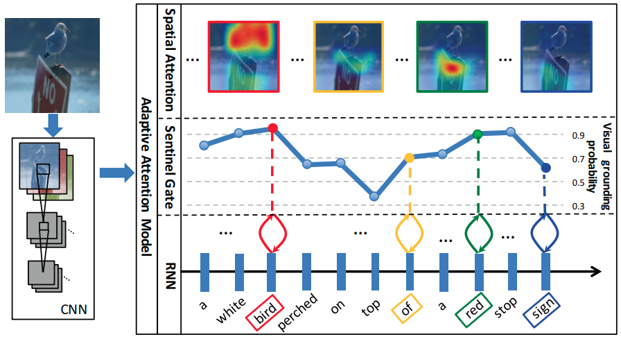
Adaptive attention with a “visual sentinel”[6] is proposed to decide when to rely on the visual signals and when to just rely on the language model.
Spatial Attention
A spatial attention (fig. (b)) is uesd to compute the context vector as:
where $g$ is the attention function, is the $d$-dimensional spatial image feature, is the hidden state of RNN at time $t$.
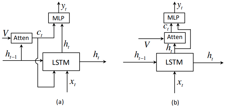
As in fig. (b), given the spatial image feature and , the context vector can be computed as:
where $\mathbb{I} \in \mathbb{R}^k$ is a vector with all elements set to 1, , are trainable parameters. $\mathbf{\alpha} \in \mathbb{R}^k$ is the attention weight over features in $\mathbf{V}$. $\mathbf{I}$ is the input image.
It uses the current hidden state rather than the previous one to generate the context vector, which can be treated as the residual visual information of current hidden state , diminishing the uncertainty or complements the informativeness of the current hidden state for next word prediction.
Adaptive Attention
Aforementioned spatial attention cannot determine when to leverage visual signals or language models. The visual sentinel vector is extended on LSTM:
where the new sentinel gate at time $t$ controls the trade-off beween the image information and decoder memory.
The new sentinel gate is computed as:
where is the attention distribution over both the spatial image feature and visual sentinel vector. In which the last element serves as the gate value .
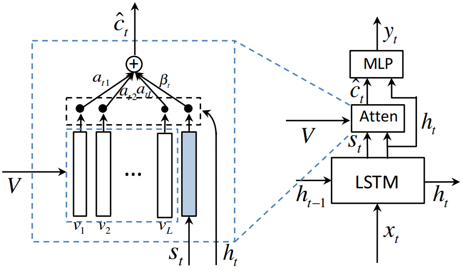
The probability over vocabulary at time $t$ is:
Semantic Compositional Networks (CVPR 2017)
Motivation: LSTM-based generation is quite limited: it only uses semantic concepts through soft attention or initialization at the first step.
Semantic Compositional Network
Semantic Compositional Networks (SCN)[7] detect the semantic concepts, i.e., tags, from each input image. It uses the $K$ most common words in the training captions to determine the vocabulary of tags, including most frequent nouns, verbs, or adjectives.
The tag detection can be cast as a multi-label classification task. Given $N$ training examples, is the label’s dummy encoding of $i$-th image, wherein 1 and 0 indicate annotation or not respectively. Let and be the image feature vector and semantic feature vector of the $i$-th image, the cost function is:
where is a $K$-dimensional vector with .
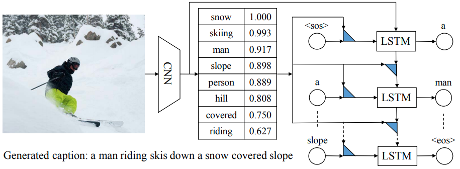
SCN-RNN
SCN injects the tag-dependent matrices:
where is the $t$-th word in the generated caption, is defined as the ‘BOS’ token, $\odot$ is the Hadamard product. Trainable parameters , , where $d$ is the hidden dimension, $d^\prime$ is the number of factors. and are shared among all captions, capturing common linguistic patterns; accounts for semantic aspects of the image captured by $\mathbf{s}$.

SCN-LSTM
SCN-RNN can be generalized using LSTM units:
where . For $\star = i,f,o,c$, we define
Training
Given image $\mathbf{I}$ and corresponding caption $\mathbf{X}$, the objective function is defined as:
Averaged objectives among all (image, caption) pairs are used during training.
Up-Down Attention (CVPR 2018)
Up-Down Attention[8] combines the bottom-up (based on Faster R-CNN[9]), a top-down attention mechanism to attend to attention at the level of objects and other salient image regions. Top-down uses the non-visual or task-specific contexts to predict an attention distribution over image regions using ResNet-101[10], whereas bottom-up proposes a set of salient image regions, wich each region represented by a pooled convolutional feature vector using Faster R-CNN.
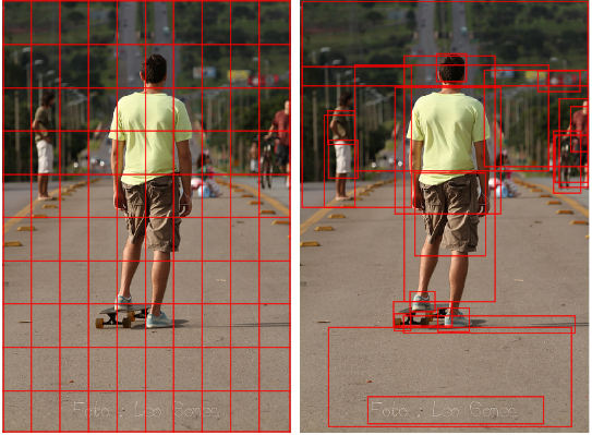
As shown in the left figure, the input regions correspond to a uniform grid of equally sized and shaped neural receptive fields, irrespective of the content of the image. In contrast, the right focuses on the objects and salient image regions for attention.
Bottom-Up attention
All regions whose class detection probability exceeds a confidence threshold are selected[9]. For each selected region $i$, is defined as the mean-pooled convolutional feature from this region.
Decoder
A top-down attention LSTM followed by a language model (LM) LSTM is used to generate captions.
Attention LSTM
Let superscript denotes the layer number, i.e., $\mathbf{h}^1$ indicates the hidden state in the first LSTM. The top-down attention LSTM receives the concatenated previous output of LM LSTM , mean-pooled image feature and the previous generated word vector , where is the word embedding matrix for vocabulary $V$, and is one-hot encoding of the input word at timestep $t$.
The output of the attention LSTM, a normalized attention weight for each of the $k$ image features at each time step $t$:
where is the input to language LSTM, are learnable parameters.
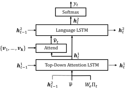
Language LSTM
The input to LM LSTM is concatated image features and attention LSTM output:
The predicted caption sequences :
where and are learnable weights and biases.
The probability of generated captions is:
Objective
Cross-entropy
Given the ground truth sequence , the corss entropy loss is:Negative expected score
where $r$ is the score function (e.g., CIDEr).
Stylized Image Captioning
StyleNet (CVPR 2017)
Motivation:
- Previous works on image captioning all generate the factual description of the image content while overlooking the style of generated captions. Stylized descriptions can greatly enrich the expressibility and attractiveness of the caption.
- Application: people always struggle to come up with an attractive title when uploading images to a social media platform. Stylized captioning can be a helpful solution.
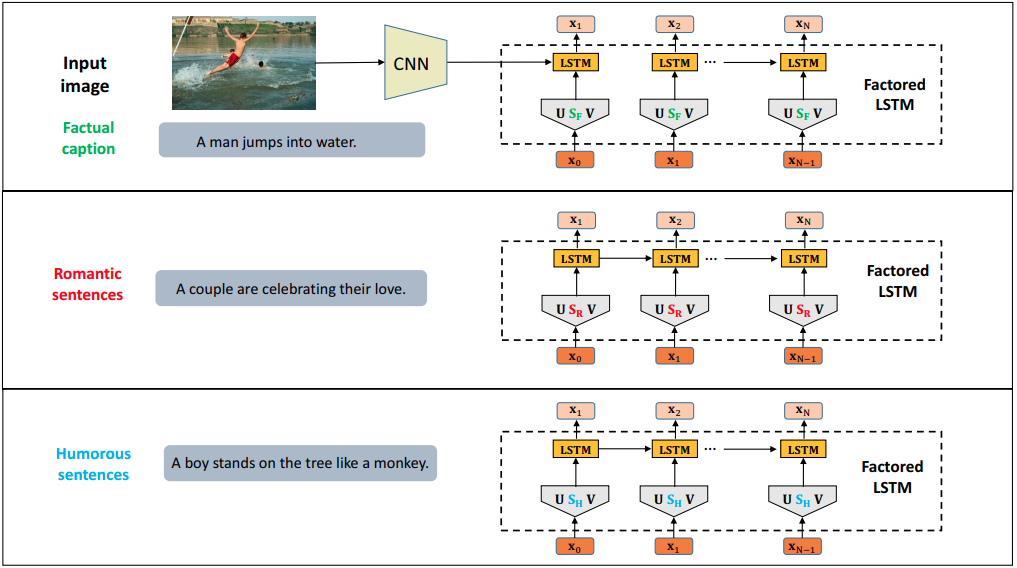
Factored LSTM
StyleNet[11] proposed the Factored LSTM to memorize the languge style pattern, by factorizing the parameters in standard LSTMs into three matrices . But it retain the weight parameters of recurrent connections , which captures the long span syntactic dependency of the text.
The Factored LSTM are defined as:
where ${ \mathbf{U}, \mathbf{V}, \mathbf{W} }$ are shared among different styles. But $\mathbf{S}$ is style-specific.
Training StyleNet
Two tasks:
- Firstly, train the factored LSTM model to generate factual captions given paired images.
- Train factored LSTM as language model on stylized language corpus, but only update the style-specific matrix $\mathbf{S}$.
SemStyle (CVPR 2018)
SemStyle[12] proposed a term generator by generating an ordered term sequence of image semantics, and a language generator trained on styled text data.

Semantic term
Given a setence , a set of rules is defined to get ordered semantic terms . The rules are as:
- Filtering non-semantic words
- lemmatization and tagging using spaCy.
- Verb abstraction. Use semantic role labeling tool SEMAFOR to annotate frames and reduce frame vocabulary.
Term generator
Use CNN+GRU to generate semantic terms collected above. The greedy search decoding is used to recover the term sequence from the conditional probabilities. Given input image $I$,
where is the ‘BOS’ token.
Language generator
A bi-GRU is used to encode the semantic terms $x$’s, and concatenate the forward and backward hidden states as outputs: . The last state is used to initialize the first hidden state of decoder: .
The context vector at step $t$ is computed with bi-linear attention:
The output uses a NLP with softmax non-linearity:
Training
Train the term generator on factual descriptions, using mean categorical cross entropy over semantic terms:
Train the language generator on both styled and descriptive sentences.
“Factual” or “Emotional” (ECCV 2018)
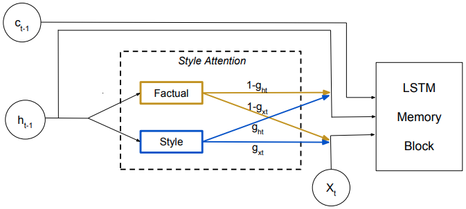
Style-factual LSTM
Two set of matrices are used in style-factual LSTM:
where style-related matrices and controls to predict word based on ($\approx 0$), or a styled word ($\approx 1$) [13].
Training
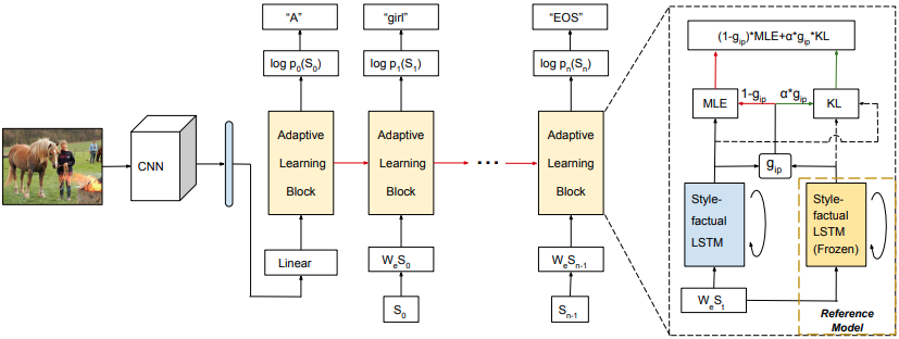
Two stages:
- At the first stage, fix and freeze the style-related matrices and . The model is trained using paired factual captioning datasets with MLE loss.
- At 2nd stage, train the model on paried stylized captioning datasets, but update and for style-factual LSTM, and fix . The loss for this stage is designed as:where and are predicted word probability distribution by the real model and the reference, represents the similarity between word probability distributions and . The term when has a higher probability to a stylized word.
Adversarial Training
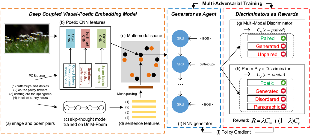
Show, Adapt and Tell (ICCV 2017)
In the source domain, given a set with paired image and ground truth sentence $\hat{\mathbf{y}}^n$. In the target domain, two separate sets are given: a set of example images and example sentences .
Captioner as an Agent
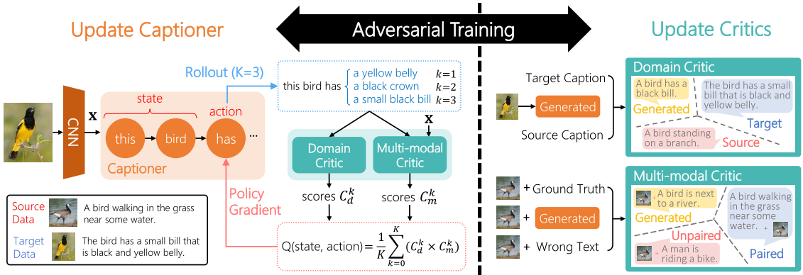
Captioner using the standard CNN-RNN architecture is treated as an agent. At time $t$, the captioner takes an action, i.e., a word , according to a stochastic policy . The total per-word loss $J(\theta)$ is minimized:
where $N$ is the number of images, is the length of the sentence , $\mathcal{L}$ indicates the cross-entropy loss. and are ground truth partial sentence and word, respectively.
The state-action function
The object function:
Since the action sapce of is huge, $M$ sentences is generated and replace expectation with the mean:
The policy gradient is:
Monte Carlo roolout is used to replace the expectation of Q function:
where are generated future words, and $K$ complete sentences are sampled with policy .
Critics
Domain critic
Domain critic (DC) model uses an encoder with a classifier. A sentence $\mathbf{y}$ is encoded using TextCNNs with highway connection, the pass to an MLP followed by a softmax to generate probability , where $l \in$ {source, target, generated}.
Training DC: the goal is to classify a sentence into source, target, and generated data.
Multi-modal critic
Multi-modal critic (MC) classifies $(\mathbf{x}, \mathbf{y})$ as “paired”, “unpaired”, or “generated” data. The model is:
where are learnable parameters, $\odot$ denotes the element-wise product, is the probabilities over three classes: paired, unpaired, and genrated data. indicates how a generated caption $\mathbf{y}$ is relevant to an image $\mathbf{x}$.
Training MC: the goal is to classify the image-sentence pair into paired, unpaired, and generated data.
Sentence reward
The sentence reward
Training algorithm
Require: captioner , domain critic , multi-modal critic , and empty set of generated sentences , and an empty set for paired image-generated-sentence .
Input: sentences , image-sentence pairs , unpaired data in source domain; sentences , images in target domain.
1, Pretrain on ;
- while $\theta$ has not converged do:
- for $i=0, \cdots, N_c$ do
- , where and ;
- Compute ;
- , where and ;
- ;
- Compute ;
- Adam update for $\eta$ for using ;
- for do
- , where and ;
- ;
- for $t=1, \cdots, T$ do
- Compute with Monte Carlo rollouts;
- Compute ;
- Adam update of $\theta$ using .
- for $i=0, \cdots, N_c$ do
Poetry generation (ACM MM 2018)
Reinforcement Learning
Self-Critical Sequence Training (CVPR 2017)
Motivation:
- Teacher-Forcing leads to the mismatch between training and testing, and exposure bias, resulting in error accumulation during generation at test time.
- While training with cross-entropy loss, discrete and non-differentiable NLP metrics such as BLEU, ROUGE, METEOR, CIDEr are evaluated at test time.
- Ideally, sequence models should be trained to avoid exposure bias and directly optimize metrics for the task at hand.
Policy Gradient
Reinforcement Learning (RL) can be used to directly optimize NLP metrics and address the exposuire bias issue, such as REINFORCE and Actor-Critic. LSTM can be treated as an agent that interacts with an external environment (state: words and image features, action: predicted words, done: “EOS”). The policy network results in an action of next word prediction. After each action, the agent updates its internal state (parameters) until generating the EOS token. The reward $r$ is the NLP metric, like CIDEr score of generated sentence by comparing with ground-truth sequences. The goal is to minimize the negative expected reward:
where and is the word sampled from the model at the time step $t$. In practive, $ \mathcal{L} (\theta)$ is typically estimated with a single sample from :
Policy gradient with REINFORCE
REINFORCE is based on the observation that the expected graident of a non-differentiable reward function:
In practice, a single MC sample from , for each training example in the minibatch:
REINFORCE with Baseline
To reduce the variance of the gradient estimate, it minus a reference reward or baseline $b$:
The baseline can be arbitrary function, as long as it does not depend on the action $w^s$ because:
This shows that the baseline does not change the expected gradient but can reduce the variance.
For each training case, it can be approximated with a single sample as:
Note if $b$ is a function of $\theta$ or $t$, this is sill valid.
The gradient is:
where is the input to the softmax function;
Self-Critical Sequence Training (SCST)
Self-Critical Sequence Training [16] applies the reward obtained by the current model under the inference mode at test time as the baseline in REINFORCE. The gradient at time step $t$ becomes:
where is the reward obtained by the current model at test time.
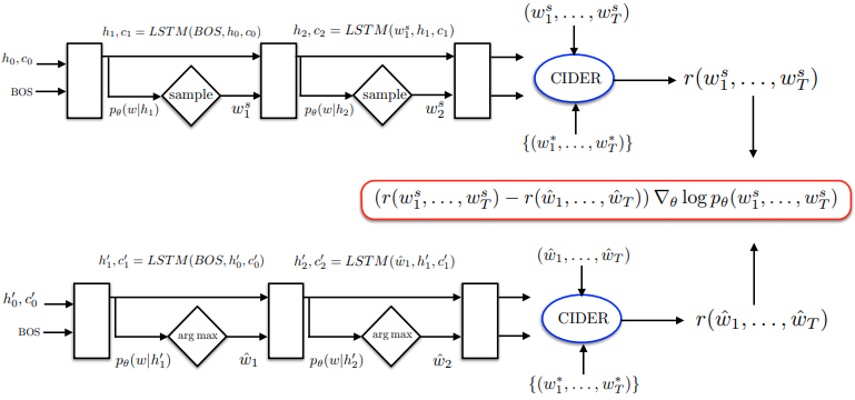
- SCST directly optimizes the true, sequence-level, evaluation metric, encouraging train/test time consistency.
- SCST avoids the usual scenario of having to learn a (context-dependent) estimate of expected future rewards as a baseline.
- In practice, it has much lower variance and is more effective on mini-batches using SGD.
- It avoids the training problems with actor-critic methods, where the actor is trained on value functions estimated by a critic rather than actual rewards.
It uses the greedy decoding:
RL with Embedding Reward (CVPR 2017)
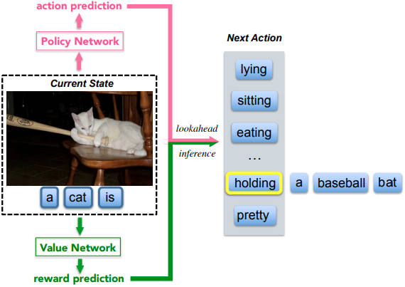
This work[17] utilized the Actor-Critic algorithm with the reward of visual-semantic embedding for image captioning. The policy and value network jointly determine the next best word at each time step. The former provides a local guidance by predicting the confidence of predicted next words, whereas the latter serves as the global and lookahead guidance by evaluating the reward value of the current state.
Policy Network
The policy network consists of standard CNN-RNN encoder-decoder architecture, with the huge vocabulary size as its action space.
Value Network
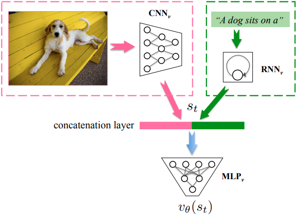
The value function is predicted by a value network .
where .
As in the figure, the value network consists of a CNN, an RNN, and an MLP, where CNN encodes the raw image $\mathbf{I}$, RNN encodes the semantic information of partially generated sentence . The concatenated representation is projected to a scalar reward from using MLP.
Visual-Semantic Embedding Reward
Give an image with feature , the reward of generated sentence $\hat{S}$ is defined to be the embedding similarity between $\hat{S}$ and $\mathbf{v}^*$:
The bidirectional ranking loss is defined as:
where $\beta$ is margin cross-validated, $(\mathbf{v}, S)$ are ground truth image-sentence pair, $S^-$ is a negetive description for image corresponding to $\mathbf{v}$, and vice-versa with $\mathbf{v}^-$.
Training
Two steps:
- Train policy network use cross entropy loss;
- Train and jointly using reinforcement learning and curriculum learning. And the value network serves as a moving baseline.
References
- 1.Vinyals, O., Toshev, A., Bengio, S., & Erhan, D. (2015). Show and tell: A neural image caption generator. 2015 IEEE Conference on Computer Vision and Pattern Recognition (CVPR), 3156-3164. ↩
- 2.Xu, K., Ba, J., Kiros, R., Cho, K., Courville, A.C., Salakhutdinov, R., Zemel, R.S., & Bengio, Y. (2015). Show, Attend, and Tell: Neural Image Caption Generation with Visual Attention. ICML. ↩
- 3.Karpathy, A., & Li, F. (2015). Deep visual-semantic alignments for generating image descriptions. CVPR. ↩
- 4.You, Q., Jin, H., Wang, Z., Fang, C., & Luo, J. (2016). Image Captioning with Semantic Attention. 2016 IEEE Conference on Computer Vision and Pattern Recognition (CVPR), 4651-4659. ↩
- 5.Chen, L., Zhang, H., Xiao, J., Nie, L., Shao, J., Liu, W., & Chua, T. (2017). SCA-CNN: Spatial and Channel-Wise Attention in Convolutional Networks for Image Captioning. 2017 IEEE Conference on Computer Vision and Pattern Recognition (CVPR), 6298-6306. ↩
- 6.Lu, J., Xiong, C., Parikh, D., & Socher, R. (2017). Knowing When to Look: Adaptive Attention via a Visual Sentinel for Image Captioning. 2017 IEEE Conference on Computer Vision and Pattern Recognition (CVPR), 3242-3250. ↩
- 7.Gan, Z., Gan, C., He, X., Pu, Y., Tran, K., Gao, J., Carin, L., & Deng, L. (2017). Semantic Compositional Networks for Visual Captioning. 2017 IEEE Conference on Computer Vision and Pattern Recognition (CVPR), 1141-1150. ↩
- 8.Anderson, P., He, X., Buehler, C., Teney, D., Johnson, M., Gould, S., & Zhang, L. (2017). Bottom-Up and Top-Down Attention for Image Captioning and Visual Question Answering. 2018 IEEE/CVF Conference on Computer Vision and Pattern Recognition, 6077-6086. ↩
- 9.Ren, S., He, K., Girshick, R.B., & Sun, J. (2015). Faster R-CNN: Towards Real-Time Object Detection with Region Proposal Networks. IEEE Transactions on Pattern Analysis and Machine Intelligence, 39, 1137-1149. ↩
- 10.He, K., Zhang, X., Ren, S., & Sun, J. (2016). Deep Residual Learning for Image Recognition. 2016 IEEE Conference on Computer Vision and Pattern Recognition (CVPR), 770-778. ↩
- 11.Gan, C., Gan, Z., He, X., Gao, J., & Deng, L. (2017). StyleNet: Generating Attractive Visual Captions with Styles. 2017 IEEE Conference on Computer Vision and Pattern Recognition (CVPR), 955-964. ↩
- 12.Mathews, A.P., Xie, L., & He, X. (2018). SemStyle: Learning to Generate Stylised Image Captions Using Unaligned Text. 2018 IEEE/CVF Conference on Computer Vision and Pattern Recognition, 8591-8600. ↩
- 13.Chen, T., Zhang, Z., You, Q., Fang, C., Wang, Z., Jin, H., & Luo, J. (2018). "Factual" or "Emotional": Stylized Image Captioning with Adaptive Learning and Attention. ECCV. ↩
- 14.Chen, T., Liao, Y., Chuang, C., Hsu, W.T., Fu, J., & Sun, M. (2017). Show, Adapt, and Tell: Adversarial Training of Cross-Domain Image Captioner. 2017 IEEE International Conference on Computer Vision (ICCV), 521-530. ↩
- 15.Liu, B., Fu, J., Kato, M.P., & Yoshikawa, M. (2018). Beyond Narrative Description: Generating Poetry from Images by Multi-Adversarial Training. ArXiv, abs/1804.08473. ↩
- 16.Rennie, S.J., Marcheret, E., Mroueh, Y., Ross, J., & Goel, V. (2016). Self-Critical Sequence Training for Image Captioning. 2017 IEEE Conference on Computer Vision and Pattern Recognition (CVPR), 1179-1195. ↩
- 17.Ren, Z., Wang, X., Zhang, N., Lv, X., & Li, L. (2017). Deep Reinforcement Learning-Based Image Captioning with Embedding Reward. 2017 IEEE Conference on Computer Vision and Pattern Recognition (CVPR), 1151-1159. ↩
