GANs are widely applied to estimate generative models without any explicit density function, which instead take the game-theoretic approach: learn to generate from training distribution via 2-player games.

Generative Adversarial Networks (GAN)

Architecture

GANs consist of two components:

Generator network $G$: try to fool the discriminator by generating real-looking images
Discriminator network $D$: try to distinguish between real and fake images

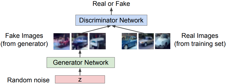
Training

Train joinly in minimax game -> minimax objective function

$\min_{G} \max_{D} V(D,G) = \mathbb{E}_{x \sim p_\text{data}(x)}\big[ \log \underbrace{D(x)}_\text{$D$ output for real data $x$} \big] + \mathbb{E}_{z \sim p_z(z)} \bigg[ \log \big(1- \underbrace{D(G(z))}_\text{$D$ output for generated fake data $G(z)$}\big) \bigg]$

where

$D$ outputs likelihood in (0,1) of real image

Discriminator $D$ aims to maximize the objective such that $D(x) \approx 1$(real) and $D(G(z)) \approx 0$ (fake).
Generator $G$ aims to minimize the objective such that $D(G(z)) \approx 1$ (to fool the $D$)

The objective is also:

Gradient ascent on discriminator $D$: $\max_{D} \bigg[ \mathbb{E}_{x\sim p_\text{data}} \log D(x) + \mathbb{E}_{z\sim p(z)} \log \big( 1-D(G(z)) \big) \bigg]$

(not work well) Gradient descent on $G$ minimizes the $D$ being correct: $\min_G \mathbb{E}_{z \sim p(z)} \log \big( 1- D(G(z)) \big)$

Problems: when samples are likely fake, the gradient the the left region of the figure is relatively flat!
Instead, gradient ascent on $G$ maximize the likelihood of $D$ being wrong $\color{red}{\max}_G \mathbb{E}_{z \sim p(z)} \color{red}{\log D(G(z))}$

Pseudocode

Minibatch SGD training

for number of training iterations do
1. for $k$ steps do
  - Sample minibatch of $m$ noise samples $\{ z^{(1)}, z^{(2)}, \cdots,z^{(m)} \}$ from noise distribution $p_g(z)$
  - Sample minibatch of $m$ examples $\{ x^{(1)}, x^{(2)}, \cdots,x^{(m)} \}$ from data generating distribution $p_\text{data}(x)$
  - Update the discriminator by ascending its stochastic gradient: $\nabla_{\theta_d} \frac{1}{m} \sum_{i=1}^m \bigg[ \log D(x^{(i)}) + \log \big( 1-D(G(z^{(i)})) \big) \bigg]$
2. Sample minibatch of $m$ noise samples $m$ noise samples $\{ z^{(1)}, z^{(2)}, \cdots,z^{(m)} \}$ from noise distribution $p_g(z)$
3. Update the $G$ by ascending its stochastic gradient: $\nabla_{\theta_g} \frac{1}{m} \sum_{i=1}^m \log \bigg(D_{\theta_d} \big( G_{\theta_g(z^{(i)})} \big) \bigg)$

Generation

After training, use $G$ to generate new images

Evaluation

Parzen-window density estimator^[9] should be avoided for evaluation.

a.k.a. Kernel Density Esitimator (KDE)
An estimator with kernel $K$ and brandwidth $h$: $\hat{p}_h (x) = \frac{1}{nh} \sum_i K \bigg( \frac{x-x_i}{h} \bigg)$
In generative model evaluation, $K$ is usually density function of standard Gaussian distribution.
Parzen-window estimator can be unreliable

The average log-likelihood^[9] is also not correlated with the sample qualities, i.e., a model have poor log-likelihood and produce great samples, or have great log-likelihood and produce poor samples.

Theoretical Results

The global optimum $p_g=p_\text{data}$

For fixed $G$, the optimal $D$ is $\begin{equation} D^*_G(x) = \frac{p_\text{data}(x)}{p_\text{data}(x) + p_g(x)} \end{equation}$

The training criteron

$\begin{align} C(G) &= \max_D (G,D) \\ &= \mathbb{E}_{x \sim p_\text{data}} \big[ \log D^*_G(x) \big] + \mathbb{E}_{z \sim p_z} \big[ \log\big(1 - D^*_G(G(z))\big) \big]\\ &= \mathbb{E}_{x \sim p_\text{data}} \big[ \log D^*_G(x) \big] + \mathbb{E}_{x\sim p_g} \big[ \log (1 - D_G^*(x)) \big]\\ &= \mathbb{E}_{x \sim p_\text{data}} \bigg[ \log \frac{p_\text{data}(x)}{p_\text{data}(x) + p_g(x)} \bigg] + \mathbb{E}_{x\sim p_g}\bigg[ \log \frac{p_g(x)}{p_\text{data}(x) + p_g(x)} \bigg] \end{align}$

The global minimum of the virtual training criterion $C(G)$ gets the value $-\log4$ iff $p_g = p_\text{data}$ . $\begin{align} C(G) &= -\log(4) + \mathbb{KL}\bigg( p_\text{data} \Vert \frac{p_\text{data} + p_g}{2} \bigg) + \mathbb{KL}\bigg( p_g \Vert \frac{p_\text{data} + p_g}{2} \bigg)\\ &= -\log(4) + 2 \cdot \text{JSD} (p_\text{data} \Vert p_g) \end{align}$

The salient difference between VAEs and GANs when using backprop:

VAEs cannot have discrete variables at the input to the generator
GANs cannot have discrete variable at the output of the generator.

Comparison

Pros:

Beautiful, sota samples!

Cons:

Trickier / unstable to train
Cannot solve inference queries such as $p(x)$, $p(z \vert x)$

Active research

Better loss function, more stable training (Wasserstein GAN, LSGAN, …)
Conditional GANs, GANs for all kinds of applications

Generative models:

PixelCNN/ PixelRNN: Explicit density model, optimizes exact likelihood, good samples. But inefficient sequential generation
VAE: Optimize variational lower bound on likelihood. Useful latent representations, inference queries. But current sample quality not the best.
GAN: Game-theoretic approach, best samples! But can be tricky and unstable to train, no inference queries.

Deep Convolutional GAN (DCGAN)

DCGAN architecture^[2]

Generator $G$ => upsampling network with fractionally-strided convolutions
Discriminator $D$ => CNN
Replace pooling layers with strided convolutions ($D$) and fractional-strided convolutions ($G$)
BatchNorm in both $G$ and $D$
Remove FC hidden layer for deeper architectures
Use ReLU activation in $G$ for all layers except for the output which uses $\tanh$
Use LeakyReLU in $D$ for all layers

Vector Arithmetic

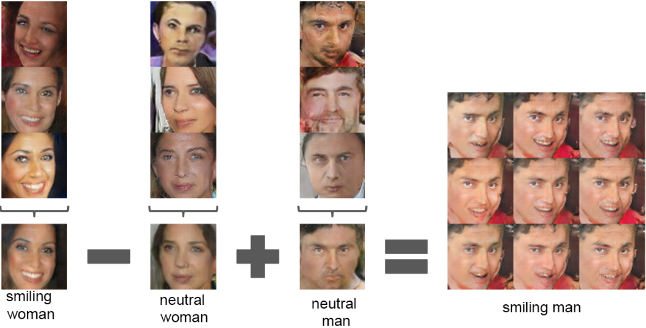
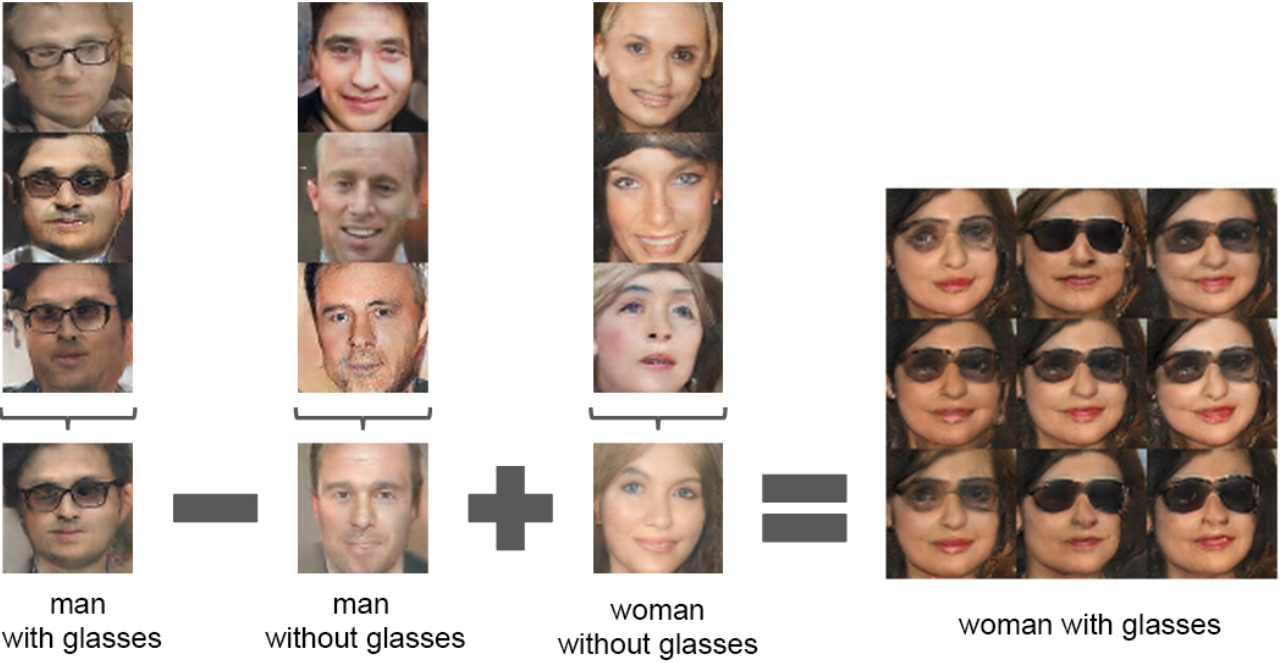
Inspired by Word2Vec that vec(“King”) - vec(“man”) + vec(“woman”) = vec(“Queen”), DCGAN found similar latent semantic representation space in $Z$ representations in the generator $G$.

The arithmetic between single samples is unstable, thus DCGAN takes the average vector of three examplars.
z(“smiling woman”) - z(“neutral woman”) + z(“neutral man”) = z(“smiling man”)
z(“man with glasses”) - z(“man without glasses”) + z(“woman without glasses”) = z(“woman with glasses”)

Improved Techniques for Training GANs

Feature Matching^[8] specifies the objective for $G$ to prevent the overtraining on the current $D$. Let $\mathbf{f(x)}$ be activations on intermediate layers of the $D$, the objective is:
$\Vert \mathbb{E}_{x \sim p_\text{data}} \mathbf{f(x)} - \mathbb{E}_{z \sim p_z(z)} \mathbf{f}(G(z)) \Vert_2^2$
Minibatch Discrimination is applied to allow the $D$ to look at multiple data in combination so as to tell the output of $G$ to be more dissimilar to each other. Let $f(\mathbf{x_i}) \in \mathbb{R}^A$ be a feature vector for input $\mathbf{x}_i$ , which is multiplied with a tensor $T \in \mathbb{R}^{A \times B \times C}$:
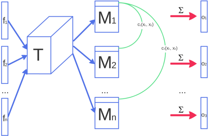
$\begin{align} M_i &= \mathbf{f(x_i)} \cdot T \in \mathbb{R}^{B \times C}\\ c_b(\mathbf{x}_i, \mathbf{x}_j) &= \exp( - \Vert M_{i,b} - M_{j,b} \Vert_{L_1})\\ o(\mathbf{x}_i)_b &= \sum_{j=1}^n c_b (\mathbf{x}_i, \mathbf{x}_j) \in \mathbb{R} \\ o(\mathbf{x}_i) &= \big[ o(\mathbf{x}_i)_1, o(\mathbf{x}_i)_2, \cdots, o(\mathbf{x}_i)_B \big] \in \mathbb{R}^B \\ o(\mathbf{X}) & \in \mathbb{R}^{n \times B} \end{align}$

Allows to incoporate side information from other samples and is superior to feature matching in the unconditional setting. This helps addressing mode collapse by allowing $D$ to detect if the generated samples are too close to each other.

Historical averaging modifies each palyer’s cost as the term
$\bigg\Vert \mathbf{\theta} - \frac{1}{t} \sum_{t=1}^t \mathbf{\theta}[i] \bigg\Vert^2$
where $\mathbf{\theta}[i]$ is the parameters at past time $i$.
One-sided label smoothing applies smoothed values like .0 or .1 as the target of 0 and 1.
$\begin{align} \text{regular $D$ cost} &= CE(\color{blue}{1.}, D(\text{data})) + CE (\color{blue}{0.}, , D(\text{samples}))\\ \text{one-sided label smooothed} &= CE(\color{red}{.9}, D(\text{data})) + CE (\color{red}{.1}, , D(\text{samples})) \end{align}$

Virtual batch normalization uses a reference batch (fixed) to compute normalization statistics and constract a batch containing the sample and reference batch.

Inception score $\exp \big( \mathbb{E}_x KL(p(y \vert \mathbb{x}) \Vert p(y) ) \big)$ has been empirically shown to be well correlated with human judgement.

Conditional GAN

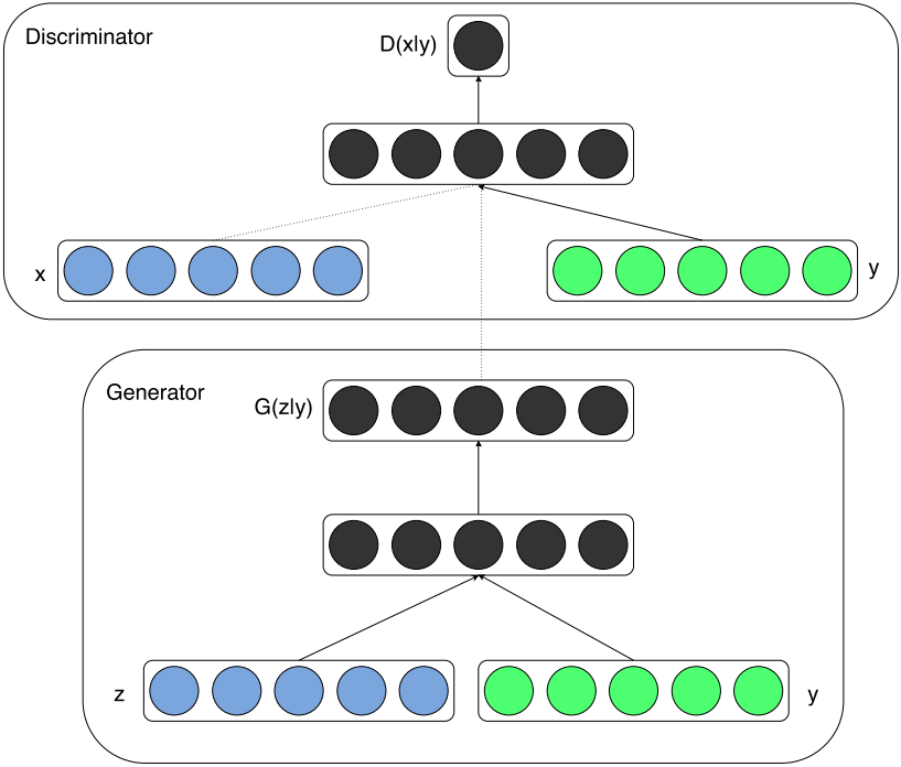
Conditional GAN^[6] feeds the input $y$ to conditional on both the generator $G$ and discriminator $D$.

In $G$, the prior input noise $p_z(z)$ and $y$ are combined in joint hidden representations;
In $D$, $x$ and $y$ are presented as inputs.

The objective function is:

$\max_{D} \bigg[ \mathbb{E}_{x\sim p_\text{data}} \log D(x \color{red}{|y}) + \mathbb{E}_{z\sim p(z)} \log \big( 1-D(G(z\color{red}{|y})) \big) \bigg]$

InfoGAN

InfoGAN ^[20] maximizes the mutual information between a small subset of the latent variables and the observation. Given the generator $G$ with both the incompressible noise $z$ and the latent code $c$, the generator becomes $G(z,c)$. InfoGAN applies the information-theoretic regularization, $i.e.$, the high mutual information (MI) between latent codes $c$ and generator distribution $G(z,c)$.

InfoGAN aims to solve the information-regularized minimax game:

$\min_G \max_D V_I (D,G) - \lambda I (c; G(z,c))$

In practice, the mutual information term $I(c; G(z,c))$ is hard to maximize directly as it requires the posterior $P(c \vert x)$. InfoGAN defines an auxiliary distribution $Q(c \vert x)$ to approximate $P(c \vert x)$:

$\begin{align} I(c; G(z,c)) &{}= H(c) - H(c \vert G(z,c)) \\ &{}= \mathbb{E}_{x \sim G(z,c)} \big[ \mathbb{E}_{c^\prime \sim P(c \vert x)} [ \log P(c^\prime \vert x) ] \big] + H(c) \\ &{}= \mathbb{E}_{x \sim G(z,c)} \big[ \underbrace{\mathbb{D}_\textrm{KL} (P(\cdot \vert x) \Vert Q(\cdot \vert x))}_{\geq 0} + \mathbb{E}_{c^\prime \sim P(c\vert x)} [ \log Q(c^\prime \vert x) ] \big] + H(c) \\ &{}\geq \mathbb{E}_{x \sim G(z,c)} \big[ \mathbb{E}_{c^\prime \sim P(c \vert x)} [ \log P(c^\prime \vert x) ] \big] + H(c) \end{align}$

The variational lower bound $L_1 (G,Q)$ of the mutual information $I(c;G(z,c))$:

$\begin{align} L_1 (G,Q) &{}= \mathbb{E}_{c \sim P(c), x\sim G(z,c)} [\log Q (c \vert x)] + H(c) \\ &{}= \mathbb{E}_{x \sim G(z,c)} \big[ \mathbb{E}_{c^\prime \sim P(c\vert x)}[\log Q(c^\prime \vert x)] \big] + H(c) \\ &{}\leq I(c; G(z,c)) \end{align}$

where $L_1$ can be maximized w.r.t. $Q$ directly and w.r.t. $G$ via the reparametrization trick. Hence $L_1 (G,Q)$ can be added to the GAN’s objectives with no changes to GAN’s training procedure.

Thus, InfoGAN defines the minimax game with a variational regularization of mutua information and a hyperparameter $\lambda$:

$\min_{G,Q} \max_D V_\textrm{InfoGAN} (D,G,Q) = V(D,G) - \lambda L_1 (C,Q)$

Wasserstein GAN (WGAN)

WGAN^[7] designed the objective function such that $G$ minimizes the Earth Mover/Wasserstein distance between data and generative distributions.
It improved the stability of learning, avoiding to balance generator $G$ and discriminator $D$’s capacity properly. It also got rid of the mode collapse.

EM distance

It applies Earth Mover (EM) distance or Wasserstein-1：

$W(\mathbb{P}_r, \mathbb{P}_g) = \inf_{\gamma \in \prod (\mathbb{P}_r,\mathbb{P}_g)} \mathbb{E}_{(x,y) \sim y} \big[ \Vert x - y \Vert \big]$

where $\prod (\mathbb{P}_r,\mathbb{P}_g)$ denotes the set of all joint distributions $\gamma(x,y)$ whose marginals are respectively $\mathbb{P}_r$ and $\mathbb{P}_g$ .
“Intuitively, $\gamma(x,y)$ indicates how much ‘mass’ must be transported from $x$ to $y$ in order to transform the distributions $\mathbb{P}_r$ into $\mathbb{P}_g$ . The EM distance is the ‘cost’ of the optimal transport plan.”^[7]
-In EM distance, the infimum $\inf$ is intractable to compute!

Thus it applies Kantorovinch-Rubinstein duality:

$W(\mathbb{P}_r, \mathbb{P}_g) = \sup_{\Vert f \Vert_L \leq 1} \mathbb{E}_{x\sim \mathbb{P}_r} [f(x)] - \mathbb{E}_{x \sim \mathbb{P}_\theta}[f(x)]$

where the supremum is over all the 1-Lipschitz functions $f: \chi \rightarrow \mathbb{R}$

$f: X \rightarrow Y$ is $K$-Lipschitz if for distance functions $d_X$ and $d_Y$ on $X$ and $Y$, $d_Y\big( f(x_1), f(x_2) \big) \leq K d_x (x_1, x_2)$

Assume that we search over a parameterized family of functions $f_w$ which $w \in \mathcal{W}$:

$\begin{align} \max_{w \in \mathcal{W}} \mathbb{E}_{x \in \mathbb{P}_r} \big[ f_w(x) \big] &\leq \sup_{\Vert f_L \Vert \leq K} \mathbb{E}_{x \sim \mathbb{P}_r} [f(x)] - \mathbb{E}_{x \sim P_g}[f(x)]\\ &=K \cdot W(\mathbb{P}_r, \mathbb{P}_g) \end{align}$

For $\mathbb{P}_g$ induced by $g_\theta (z)$ we can backprop through $\mathbb{E}_{x \sim P_r}[f_w(x)]$ : $- \mathbb{E}_{z \sim p(z)} [\nabla_\theta f_w (g_\theta (z))]$

WGAN pseudocode

Given:

$\alpha=1e-5$: learning rate
$c=0.01$: clipping hyperparameter
$m=64$: batch size
$n_\text{critic}=5$: the # of iterations of the critic per generator iteration
$w_0$ : initial critic parameters; $\theta_0$ : initial generator’s parameters

while $\theta$ has not converged do

for $t=0,\cdots, n_\text{critic}$ do:
1. Sample $\{x^{(i)}\}_{i=1}^m \sim \mathbb{P}_r$ , a batch from the real data
2. Sample $\{z^{(i)}\}_{i=1}^m \sim p(z)$ a batch of prior samples
3. Update $g_w \leftarrow \nabla_w [\color{red}{ \frac{1}{m} \sum_{i=1}^m f_w(x^{(i)}) - \frac{1}{m} \sum_{i=1}^m f_w \big( g_\theta (z^{(i)}) \big)} ]$
4. Update $w \leftarrow w + \alpha \cdot \text{RMSProp}(w, g_w)$
5. Update $w \leftarrow \text{clip}(w, -c, c)$
Sample $\{z^{(i)}\}_{i=1}^m \sim p(z)$ a batch of prior samples
Update $g_\theta \leftarrow \color{blue}{ - \nabla_\theta \frac{1}{m} \sum_{i=1}^m f_w \big( g_\theta (z^{(i)}) \big) }$
Update $\theta \leftarrow \theta - \alpha \cdot \text{RMSProp}(\theta, g_\theta)$

Results

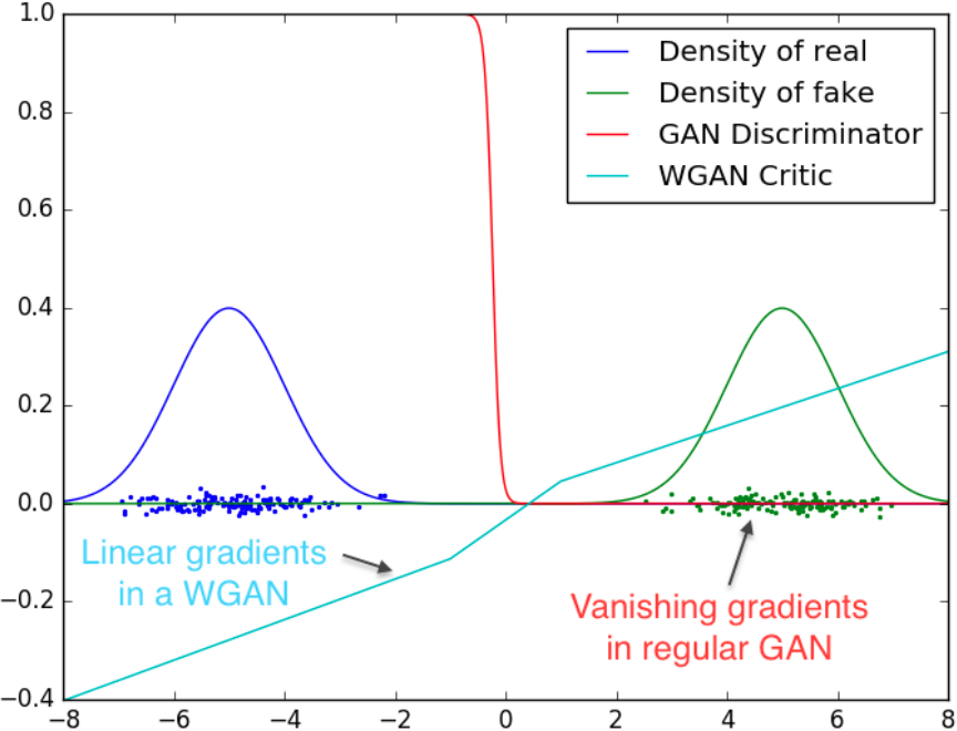
It can be seen that the gradient of regular GAN’s discriminator could get vanishing gradients whereas the WGAN’s critic cannot saturate and converge to a linear function with gradients everywhere.

Momentum-based optimizer like Adam perform worse since the loss for the critic is non-stationary, whereas RMSProp is known to perform well even on very non-stationary problems.
No mode collapse has been evidenced during WGAN experiments.

WGAN-GP

Problems of WGAN:

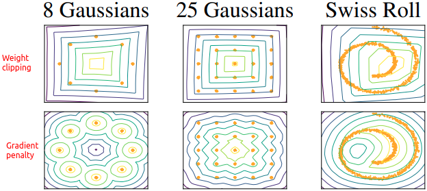
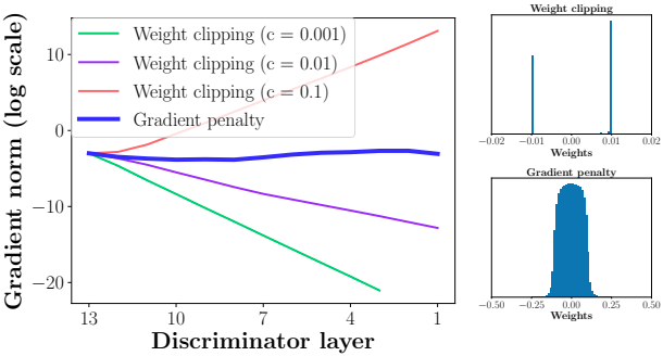
the weight clipping for $k$-Lipshitz constraint biases the $D$ towards much simpler functions.
“It is observed that our NNs try to attain the maximum gradient norm $k$ and end up learning extremely simple functions”^[10] (see figures below).

Gradient Penalty

The gradient penalty^[10] (WGAN-GP) is an alternative to implement the Lipschitz constraints. “The differentiable function is 1-Lipschtiz iff it has gradients with norm at most 1 everywhere”^[10].

The new objective is:

$L = \underbrace{\mathbb{E}_{\mathbf{\tilde{x}} \in \mathbb{P}_g} \big[ D(\color{red}{\mathbf{\tilde{x}}}) - \mathbb{E}_{\mathbf{x} \sim \mathbb{P}_r}[D(\color{blue}{\mathbf{x}})] \big]}_\textit{original critic loss} + \underbrace{\lambda \mathbb{E}_{\mathbf{\hat{x}} \in \mathbb{P}_{\mathbf{\hat{x}}}} \big[ ( \Vert \nabla_{\mathbf{\hat{x}}} D( \color{orange}{ \mathbf{\hat{x}} }) \Vert_2 -1 )^2 \big] }_{\color{green}{\textit{gradient penalty}}}$

Sample distribution: define $\mathbb{P}_\mathbf{\hat{x}}$ sampling uniformly along straight lines between pairs $\hat{\mathbf{x}}$ and $\mathbf{x}$ sampled from the data distribution $\mathbb{P}_r$ and generator distribution $\mathbb{P}_g$ , i.e.: $\color{orange}{ \hat{\mathbf{x}} } \leftarrow \epsilon \color{blue}{\mathbf{x}} + (1-\epsilon) \color{red}{\mathbf{\tilde{x}}}$

Pseudocode

Given:

gradient penalty coefficient $\lambda = 10$
# of critic iterations per generator iteration $n_\text{critic}$
batch size $m$
Adam hyperparameters $\alpha=1e-3, \beta_1=0, beta_2 = 0.9$
Initial critic parameters $w_0$ , initial generator parameters $\theta_0$

while $\theta$ has not converged do

for do:
1. for $i=1, \cdots, m$ do:
  1. Sample real data $\mathbf{x} \in \mathbb{P}_r$ , latent variable $z \in p(z)$ , a random number $\epsilon \sim U[0,1]$
  2. forward pass of $G$: $\tilde{\mathbf{x}} \leftarrow G_\theta(z)$
  3. $ \color{orange}{ \hat{\mathbf{x}}} \leftarrow \epsilon \color{blue}{\mathbf{x}} + (1-\epsilon) \color{red}{\mathbf{\tilde{x}}} $
  4. Objective: $L^{(i)} \leftarrow D_w(\color{red}{\tilde{\mathbf{x}}}) - D_w(\color{blue}{\mathbf{x}}) + \color{green}{ \lambda( \Vert \nabla_{\color{orange}{ \mathbf{\hat{x}} }} D_w( \color{orange}{ \mathbf{\hat{x}} }) \Vert_2 -1)^2 }$
2. Update $D$: $w \leftarrow(\nabla_w \frac{1}{m}\sum_{i=1}^m L^{(i)}, w, \alpha, \beta_1, \beta_2 )$
Sample a batch of latent variables $\{z^{(i)}\}_{i=1}^m \sim p(z)$
Update $G$: $\theta \leftarrow \text{Adam}(\nabla_\theta \frac{1}{m}\sum_{i=1}^m - D_w(G_\theta (z)), \theta, \alpha, \beta_1, \beta_2 )$

Spectral Normalization GAN (SN-GAN)

Spectral normalization^[11] is a novel weight normalization method to stablize the training of discriminator $D$.

For a linear layer $g(\mathbf{h})= W \mathbf{h}$ , the norm is given by:

$\begin{align} \Vert g \Vert_\text{Lip} &= \sup_{\mathbf{h}} \sigma (\nabla g(\mathbf{h})) \\ & = \sup_{\mathbf{h}} \sigma (W) \\ & = \sigma (W) \end{align}$

If the Lipchiz norm of the activation function $\Vert a_l \Vert_\text{Lip} = 1$ , we can use the inequality $\Vert g_1 \circ g_2 \Vert_\text{Lip} \leq \Vert g_1 \Vert_\text{Lip} \cdot \Vert g_2 \Vert_\text{Lip}$ to observe the following bound on $\Vert f \Vert_\text{Lip}$ :

$\begin{align} \Vert f \Vert_\text{Lip} &\leq \Vert (\mathbf{h} \mapsto W^{L+1}\mathbf{h}_L) \Vert_\text{Lip} \cdot \Vert a_L \Vert_\text{Lip} \cdot \Vert (\mathbf{h}_{L-1} \mapsto W^{L}\mathbf{h}_{L-1}) \Vert_\text{Lip} \\ & \cdots \Vert a_1 \Vert_\text{Lip} \cdot \Vert (\mathbf{h}_0 \mapsto W^{1}\mathbf{h}_0) \Vert_\text{Lip} \\ &= \prod_{l=1}^{L+1} \Vert (\mathbf{h}_{l-1} \mapsto W^l \mathbf{h}_{l-1}) \Vert_\text{Lip} \\ & = \prod_{l=1}^{L+1} \sigma (W^l) \end{align}$

Our spectral normalization normalizes the spectral norm of the weigth matrix $W$ so that it satisfies the Lipschitz constraint $\sigma(W)=1$:

$\bar{W}_\text{SN} (W) := \frac{W}{\sigma(W)}$

Projection Discriminator

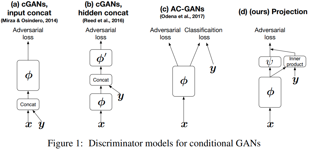
^[14] proposed a novel projection based discriminator to incorporate conditional information into the $D$ of GANs that respects the role of the conditional information.

Self-Attention GAN (SAGAN)

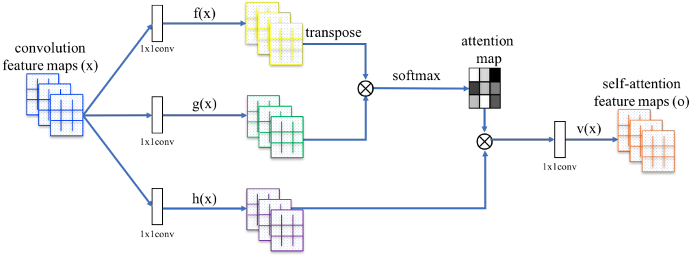
SA-GAN^[17] applies self-attention op to capture the long0range depdencies in images, whereas conventional convolution op learns the information in a local neighborhood which requires deep layers to model larger receptive regions.

Self-attention

Given images features from prev layer $\mathbf{x} \in \mathbb{R}^{C \times N}$ , firstly transform into two feature spaces $f$, $g$:

$\begin{align} f(\mathbf{x}) &= \mathbf{W}_f(\mathbf{x}) & \rightarrow \text{Q}\\ g(\mathbf{x}) &= \mathbf{W}_g(\mathbf{x}) & \rightarrow \text{K} \\ h(\mathbf{x_i}) &= \mathbf{W}_h(\mathbf{x_i}) & \rightarrow \text{V} \end{align}$

Thus,

$\begin{align} s_{ij} &= f(\mathbf{x}_i)^\top g(\mathbf{x}_j) & \\ \beta_{ji} &= \frac{\exp (s_{ij})}{\sum_{i=1}^N \exp (s_{ij})} & \text{attn weights} \\ \mathbf{c_j} & = \sum_{i=1}^N \beta_{j,i} \mathbf{h} (\mathbf{x_i}) & \text{Self attn}\\ \mathbf{o_j} &= \mathbf{W_v} \mathbf{c_j} & \text{post transformation} \end{align}$

where $\{ \mathbf{W_g, W_f, W_h} \} \in \mathbb{R}^{\bar{C} \times C}$ , $\mathbf{W}_v \in \mathbb{R}^{C \times \bar{C}}$ are 1x1 convolutions.
$C$ is the # of channels, $N$ is the # of feature locations

Further, a scale parameter are applied on the attention layer output:

$\mathbf{y_i} = \gamma \mathbf{o_i} + \mathbf{x_i}$

where $\gamma$ is a learnable scalar and is initialized as 0.

Hinge adversarial loss

SAGAN applies the hinge adversarial loss (^[13])

$\begin{align} L_D &= - \mathbb{E}_{(x,y) \sim p_\text{data}} [\min(0, -1+ D(x,y))] - \mathbb{E}_{z \sim p_z, y \sim p_\text{data}} [\min (0, -1-D(G(z), y))] \\ L_G &= - \mathbb{E}_{z \sim p_z, y \sim p_\text{data}} D(G(z), y) \end{align}$

Stablizing techniques

Spectral normalization ^[11]
two timescale update rule (TTUR) ^[12]

BigGAN

Large batch size, model size
Fuse class information at all levels (cGAN)
Hinge loss
Orthonormal regularization & Truncation trick

BigGAN ^[18] applies onthogonal regularization to directly enforces the orthogonality condition:

$\begin{align} R_\beta (W) &= \beta \Vert W^\top W - I \Vert_F^2 \\ R_\beta (W) &= \beta \Vert W^\top W \odot (\mathbf{1} - I) \Vert_F^2 \end{align}$

BigGAN architecture: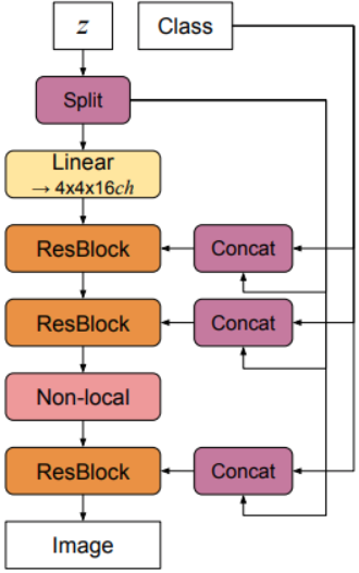

StyleGAN

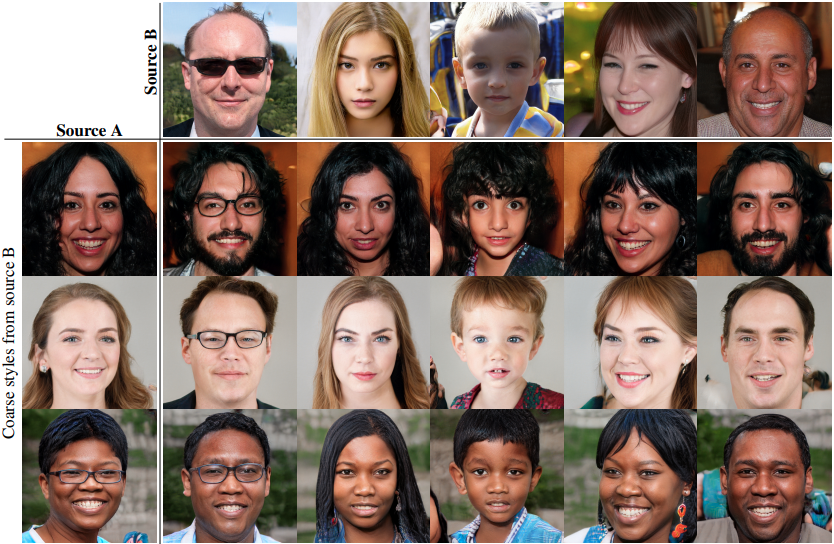
StyleGAN^[19] automatically learned unsupervised separation of high-level attributes (e.g., pose and identity when trained on human faces) and stocastic variation in generation.

Given a latent code $\mathbf{z}$ in the input latent space $\mathcal{Z}$, a non-linear mapping network $f: \mathcal{Z} \rightarrow \mathcal{W}$ first produces $\mathbf{w} \in \mathcal{W}$. Here $f$ is an 8-layer MLP.
The learned affine transformations then specialize $\mathbf{w}$ to styles $\mathbf{y}= (\color{blue}{\mathbf{y}_s}, \color{red}{\mathbf{y}_b)}$ that control the adaptive instance normalization (AdaIN):
$\text{AdaIN}(\mathbf{x}_i, \mathbf{y}) = \color{blue}{\mathbf{y}_s} \frac{\mathbf{x}_i - \mu(\mathbf{x}_i)}{\sigma (\mathbf{x}_i)} + \color{red}{\mathbf{y}_b}$
where each feature map $\mathbf{x}_i$ is normalized separately, and then scaled and biased using learned style $\mathbf{y}$.
The explicit noise inputs are broadcast to all feature maps using learned per-feature scaling factors and then added to the convolution output.

References

1.Goodfellow, I.J., Pouget-Abadie, J., Mirza, M., Xu, B., Warde-Farley, D., Ozair, S., Courville, A.C., & Bengio, Y. (2014). Generative Adversarial Networks. ArXiv, abs/1406.2661. ↩
2.Radford, A., Metz, L., & Chintala, S. (2015). Unsupervised Representation Learning with Deep Convolutional Generative Adversarial Networks. CoRR, abs/1511.06434. ↩
3.Goodfellow, I.J. (2017). NIPS 2016 Tutorial: Generative Adversarial Networks. ArXiv, abs/1701.00160. ↩
4.cs236 notes ↩
5.cs231 slides ↩
6.Mirza, M., & Osindero, S. (2014). Conditional Generative Adversarial Nets. ArXiv, abs/1411.1784. ↩
7.Arjovsky, M., Chintala, S., & Bottou, L. (2017). Wasserstein GAN. ArXiv, abs/1701.07875. ↩
8.Salimans, T., Goodfellow, I.J., Zaremba, W., Cheung, V., Radford, A., & Chen, X. (2016). Improved Techniques for Training GANs. ArXiv, abs/1606.03498. ↩
9.Theis, L., Oord, A.V., & Bethge, M. (2015). A note on the evaluation of generative models. CoRR, abs/1511.01844. ↩
10.Gulrajani, I., Ahmed, F., Arjovsky, M., Dumoulin, V., & Courville, A.C. (2017). Improved Training of Wasserstein GANs. NIPS. ↩
11.Miyato, T., Kataoka, T., Koyama, M., & Yoshida, Y. (2018). Spectral Normalization for Generative Adversarial Networks. ArXiv, abs/1802.05957. ↩
12.Heusel, M., Ramsauer, H., Unterthiner, T., Nessler, B., & Hochreiter, S. (2017). GANs Trained by a Two Time-Scale Update Rule Converge to a Local Nash Equilibrium. NIPS. ↩
13.Lim, J.H., & Ye, J.C. (2017). Geometric GAN. ArXiv, abs/1705.02894. ↩
14.Miyato, T., & Koyama, M. (2018). cGANs with Projection Discriminator. ArXiv, abs/1802.05637. ↩
15.Zhao, J.J., Mathieu, M., & LeCun, Y. (2016). Energy-based Generative Adversarial Network. ArXiv, abs/1609.03126. ↩
16.Nowozin, S., Cseke, B., & Tomioka, R. (2016). f-GAN: Training Generative Neural Samplers using Variational Divergence Minimization. ArXiv, abs/1606.00709. ↩
17.Zhang, H., Goodfellow, I.J., Metaxas, D.N., & Odena, A. (2018). Self-Attention Generative Adversarial Networks. ArXiv, abs/1805.08318. ↩
18.(BigGAN) Brock, A., Donahue, J., & Simonyan, K. (2018). Large Scale GAN Training for High Fidelity Natural Image Synthesis. ArXiv, abs/1809.11096. ↩
19.Karras, T., Laine, S., & Aila, T. (2018). A Style-Based Generator Architecture for Generative Adversarial Networks. CVPR. ↩
20.Chen, Xi, et al. Infogan: Interpretable representation learning by information maximizing generative adversarial nets. Advances in neural information processing systems. 2016. ↩