This is a concise introduction of Variational Autoencoder (VAE).

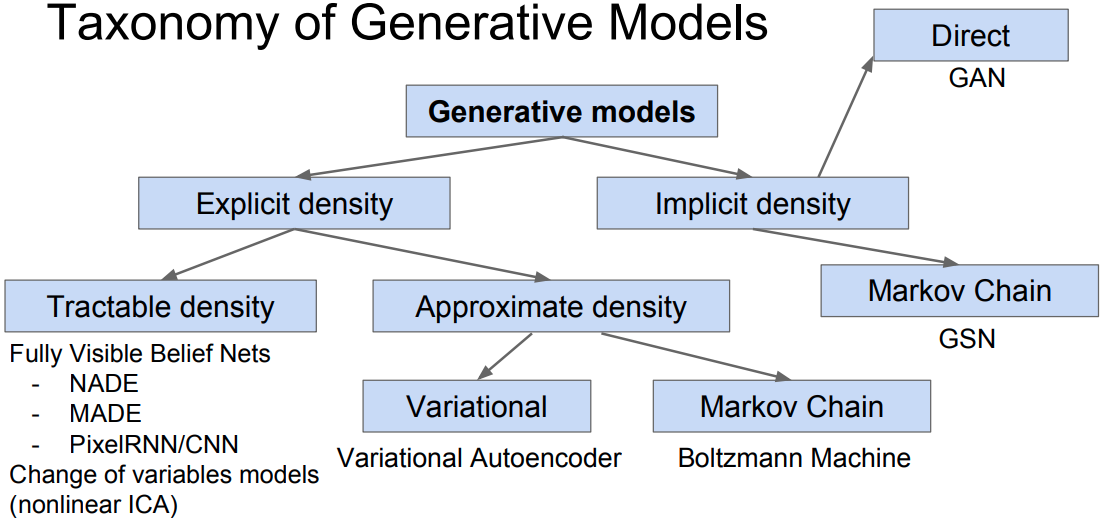
Background

PixelCNN define tractable density function with MLE:
$p(\theta) = \prod_{i=1}^n p_\theta (x_i \vert x_1, \cdots, x_{i-1})$
VAE define the intractable density function with latent $\mathbf{z}$:
$p(\theta) = \color{red}{\int} p_\theta (z) p_\theta (x \vert z) dz$

This cannot directly optimize, VAEs derive and optimize the lower bound on likelihood instead.

Autoencoder

Autoencoder (AE) encodes the inputs into latent representations $\mathbf{z}$ with dimension reduction to capture meaningful factors of variation in data. Then employ $\mathbf{z}$ to reconstruct original data by autoencoding itself.

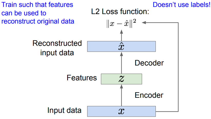
After training, throw away the decoder and only retain the encoder.
Encoder can be used to initialize the supervised model on downstream tasks.

Variational Autoencoder

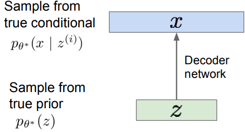
Assume training data $\{ x^{(i)}\}_{i=1}^N$ is generated from underlying unobserved (latent) representation $\mathbf{z}$.

Intuition:

$\mathbf{x}$ -> image
$\mathbf{z}$ -> latent factors used to generate $\mathbf{x}$: attributes, orientation, pose, how much smile, etc. Choose prior $p(z)$ to be simple, e.g. Gaussian.

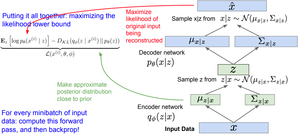
Training

Problem

Intractable integral to MLE of training data:

$p(\theta) = \color{red}{\int} \color{green}{\overbrace{p_\theta (z)}^{\checkmark\text{Gaussian prior}}} \color{green}{\underbrace{p_\theta (x \vert z)}_{\checkmark\text{decoder NN}}} dz$

where it is intractable to compute $p(x \vert z)$ for every $z$, i.e. integral. The intractability is marked in red.

Thus, the posterior density is also intractable due to the intractable data likelihood:

$p_\theta (z \vert x) = \frac{ \color{green}{p_\theta (x \vert z) p_\theta (z)}}{ \color{red}{p_\theta (x)}}$

VAE Decoder^[5]

Solution

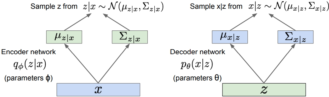
Encoder -> “recognition / inference” networks.

Define encoder network $q_\phi (z \vert x)$ that approximates the intractable true posterior $p_\theta(z \vert x)$ . VAE makes the variational approximate posterior be a multivariate Gaussian with diagonal covariance for data point $\mathbf{x}^{(i)}$: $\log q_\phi (\mathbf{z} \vert \mathbf{x}^{(i)}) = \log \mathcal{N} (\mathbf{z}; \mathbf{\mu}^{(i)}, \mathbf{\sigma}^{2(i)}\mathbf{I})$

where

For Gaussian MLP encoder or decoder^[4], $\begin{align} \mu &= \mathbf{W_4 h + b_4} \\ \log \sigma^2 &= \mathbf{W_5 h + b_5} \\ h &= \tanh (\mathbf{W_3 z + b_3}) \end{align}$

Use NN to model $\log \sigma^2$ instead of $\sigma^2$ is because that $\log \sigma^2 \in (-\infty, \infty)$ whereas $\sigma^2 \geq 0$

Decoder -> “generation” networks $p_\theta (x \vert z)$

$\begin{align} \log p_\theta (x^{(i)}) &= \mathbb{E}_{z \sim q_\phi (z \vert x^{(i)})} \bigg[ \log p_\theta (x^{(i)}) \bigg] & p_\theta (x^{(i)}) \text{ does not depend on }z \\ &= \mathbb{E}_z \bigg[ \log \frac{p_\theta (x^{(i)} \vert z) p_\theta (z)}{p_\theta (z \vert x^{(i)})} \bigg] & \text{Bayes rule} \\ &= \mathbb{E}_z \bigg[ \log \frac{p_\theta(x^{(i)} \vert z) p_\theta (z)}{p_\theta (z \vert x^{(i)})} \frac{q_\phi (z \vert x^{(i)})}{q_\phi (z \vert x^{(i)})} \bigg] & \text{multiply by constant} \\ &= \mathbb{E}_z \bigg[ \log p_\theta (x^{(i)} \vert z)\bigg] - \mathbb{E}_z \bigg[\log \frac{q_\phi (z \vert x^{(i)})}{p_\theta (z)} \bigg] + \mathbb{E}_z \bigg[ \log \frac{q_\phi (z \vert x^{(i)})}{p_\theta (z \vert x^{(i)})} \bigg] & \text{logarithms} \\ &= \underbrace{ \mathbb{E}_z \bigg[ \log \color{green}{\overbrace{p_\theta (x^{(i)} \vert z)}^\text{decoder}} \bigg] - \mathbb{KL} \big( \color{blue}{ \overbrace{q_\phi (z \vert x^{(i)})}^\text{encoder}} \| \color{blue}{\overbrace{p_\theta (z)}^{z\,\text{prior}} } \big) }_{\mathcal{L}(x^{(i)}, \theta, \phi)} + \underbrace{\mathbb{KL} \big( q_\phi(z \vert x^{(i)}) \| \color{red}{ \overbrace{p_\theta (z \vert x^{(i)})}^{\text{intactable!}} } \big)}_{\geq 0} \end{align}$

The first RHS term represents tractable lower bound $\mathcal{L}(x^{(i)}, \theta, \phi)$ , wherein $p_\theta (x \vert z)$ and $\mathbb{KL}$ terms are differentiable.
Thus, the variational lower bound (ELBO) is derived： $\log p_\theta (x^{(i)}) \geq \mathcal{L}(x^{(i)}, \theta, \phi)$
Training: maximize lower bound $\theta^*, \phi^* = \arg\max_{\theta, \phi} \sum_{i=1}^N \mathcal{L}(x^{(i)}, \theta, \phi)$

$\mathcal{L}(x^{(i)}, \theta, \phi) = \mathbb{E}_z \bigg[ \log \color{green}{\overbrace{p_\theta (x^{(i)} \vert z)}^\text{decoder}} \bigg] - \mathbb{KL} \big( \color{blue}{ \overbrace{q_\phi (z \vert x^{(i)})}^\text{encoder}} \| \color{blue}{\overbrace{p_\theta (z)}^{z\,\text{prior}} } \big)$

where

the fist term $\mathbb{E}_z \bigg[ \log \color{green}{p_\theta (x^{(i)} \vert z)} \bigg]$ : reconstruct the input data. It is a negative reconstruction error.
the second term $\mathbb{KL} \big( \color{blue}{q_\phi (z \vert x^{(i)})} \| \color{blue}{p_\theta (z)} \big)$ make approximate posterior distribution close to the prior. It acts as a regularizer.

The derived estimator when using isotropic multivariate Gaussian $p_\theta(\mathbf{z})=\mathcal{N}(\mathbf{z}; \mathbf{0,I})$ :

$\mathcal{L}(\theta, \phi;x^{(i)}) \simeq \frac{1}{2} \sum_{j=1}^D\bigg( 1+ \log((\sigma^{(i)}_j)^2) - (\mu^{(i)}_j)^2 - (\sigma_j^{(i)})^2 \bigg) + \frac{1}{L} \sum_{l=1}^L \log p_\theta (\mathbf{x}^{(i)} \vert \mathbf{z}^{(i,l)})$

where $\mathbf{z}^{(i,l)} = \mu^{i} + \sigma^{(i)} \odot \epsilon^{(l)}$ and $\epsilon^{(l)} \sim \mathcal{N}(0, \mathbf{I})$ , $\mu_j$ and $\sigma_j$ denote the $j$-th element of mean and variance vectors.

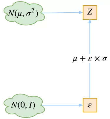
Reparameterization trick

Given the deterministic mapping $\mathbf{z}= g_\phi (\epsilon, x)$ , we know that

$q_\phi (\mathbf{z} \vert \mathbf{x})\prod_i dz_i = p(\mathbf{\epsilon})\prod_i d\epsilon_i$

Thus,

$\begin{align} \int q_\phi (\mathbf{z \vert x}) f(\mathbf{z})d\mathbf{z} &= \int p(\mathbf{\epsilon}) f(g_\phi(\mathbf{\epsilon}, \mathbf{x})) d\mathbf{\epsilon} & \\ & \simeq \frac{1}{L} \sum_{l=1}^L f(g_\phi (\mathbf{x}, \epsilon^{(l)})) & \text{where }\epsilon^{(l)}\sim p(\epsilon) \end{align}$

Take the univariate Gaussian case for example: $z \sim p(z \vert x) = \mathcal{N}(\mu, \sigma^2)$, the valid reparameterization is: $z = \mu + \sigma \epsilon$, where the auxiliary noise variable $\epsilon \sim \mathcal{N}(0,1)$.
Thus,

$\begin{align} \mathbb{E}_{\mathcal{N}(z;\mu,\sigma^2)} [f(z)] &= \mathbb{E}_{\mathcal{N}}[f(\mu+ \sigma \epsilon)] & \\ \end{align}$

Generation

After training, remove the encoder network, and use decoder network to generate.
Sample $z$ from prior as the input!
Diagonal prior on $z$ -> independent latent variables!

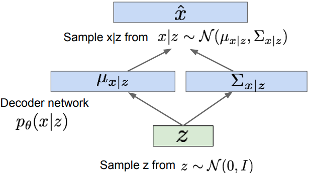
Different dimensions of $z$ encode interpretable factors of variation.
Good feature representation that can be computed using $q_\phi (z \vert x)$

Pros & cons

Probabilistic spin to traditional autoencoders => allows generating data
Defines an intractable density => derive and optimize a (variational) lower bound

Pros:

Principles approach to generative models
Allows inference of $q(z \vert x)$, can be useful feature representation for downstream tasks

Cons:

Maximizes lower bound of likelihood: okay, but not as good evalution as PixelRNN / PixelCNN！
loert quality compared to the sota (GANs)

Variational Graph Auto-Encoder (VGAE)

Definition

Given an undirected, unweighted graph $\mathcal{G}=(\mathcal{V}, \mathcal{E})$ with $N=|V|$ nodes, the ajacency matrix $\mathbf{A}$ with self-connection (i.e., the diagonal is set to 1), degree matrix $\mathbf{D}$, stochastic latent variable $\mathbf{z}_i$ in matrix $\mathbf{Z} \in \mathbb{R}^{N \times F}$, node features $\mathbf{X} \in \mathbb{R}^{N \times D}$. ^[7]

Inference model

Apply a 2-layer Graph Convolutional Networks (GCN) to for parameterization:

$\begin{align} q(\mathbf{Z} \vert \mathbf{X}, \mathbf{A}) &= \prod_{i=1}^N q(\mathbf{z}_i \vert \mathbf{X}, \mathbf{A}) \\ q(\mathbf{z}_i \vert \mathbf{X}, \mathbf{A}) &= \mathcal{N}(\mathbf{z}_i \vert \mathbf{\mu}_i, \text{diag}(\mathbf{\sigma}_i^2)) \end{align}$

where

Mean: $\mu = \text{GCN}_\mu (\mathbf{X}, \mathbf{A})$
Variance: $\log \sigma = \text{GCN}_\sigma (\mathbf{X}, \mathbf{A})$

The two-layer GCN is defined as $\text{GCN}(\mathbf{X}, \mathbf{A}) = \tilde{\mathbf{A}} \text{ReLU}(\tilde{\mathbf{A}}\mathbf{X}\mathbf{W}_0)\mathbf{W}_1$
where $\tilde{\mathbf{A}} = \mathbf{D}^{-1/2} \mathbf{A}\mathbf{D}^{-1/2}$ is the semmetrically normalized adjacency matrix.

Generative model

The generative model applies an inner product between latent variables:

$\begin{align} p(\mathbf{A}\vert \mathbf{Z}) &= \prod_{i=1}^N \prod_{j=1}^N p(A_{ij} \vert \mathbf{z}_i, \mathbf{z}_j) \\ p(A_{ij}=1 \vert \mathbf{z}_i, \mathbf{z}_j)) &= \sigma(\mathbf{z}_i^\top \mathbf{z}_j) \end{align}$

where $A_{ij}$ are elements of ajacency matrix $\mathbf{A}$ and $\sigma(\cdot)$ represents the sigmoid function.

Learning

Optimize the variational lower bound (ELBO) $\mathcal{L}$ w.r.t the variational parameters $\mathbf{W}_i$ :

$\mathcal{L} = \mathbb{E}_{q(\mathbf{Z} \vert \mathbf{X},\mathbf{A})} \big[\log p(\mathbf{A} \vert \mathbf{Z})\big] - \mathbb{KL}\big[q(\mathbf{Z} \vert \mathbf{X}, \mathbf{A}) \Vert p(\mathbf{Z})\big]$

where the Gaussian prior $p(\mathbf{Z}) = \prod_I p(\mathbf{z}_i) = \prod_i \mathcal{N}(\mathbf{z}_i \vert 0, \mathbf{I})$

References

1.Stanford cs231n: Generative models ↩
2.I. Goodfellow et. al, Deep Learning ↩
3.Goodfellow, I. (2016). Tutorial: Generative adversarial networks. In NIPS. ↩
4.Kingma, D. P., & Welling, M. (2013). Auto-encoding variational bayes. arXiv preprint arXiv:1312.6114. ↩
5.Doersch, C. (2016). Tutorial on Variational Autoencoders. ArXiv, abs/1606.05908. ↩
6.cs236 VAE notes ↩
7.Kipf, T., & Welling, M. (2016). Variational Graph Auto-Encoders. ArXiv, abs/1611.07308. ↩