Likelihood-based Generative Models II: Flow Models

Flow models are used to learn continuous data.

Discrete autoregressive models tractably learn the joint distribution by decomposing it into a product of conditionals using the probability chain rule according to a fixed ordering over dimensions.

The sequential nature limits its computational efficiency:

1. its sampling procedure is sequential and non-parallelizable;
2. there is no natural latent representation associated with autoregressive models.

To sum up:

• Pros:
  • fast evaluation of p(x)
  • great compression performance
  • good samples with carefully designed dependency structure
• Cons:
  • slow sampling (without significant engineering)
  • discrete data only

Flows explanation

Ideas: instead of using a pdf over $\mathbf{x}$, work with a flow from $\mathbf{x}$ to $\mathbf{z}$

Flows in 1D

Flow from $\mathbf{x}$ to $\mathbf{z}$ : an invertible differentiable mapping $f$ from $\mathbf{x}$ (data) to $\mathbf{z}$ (noise):

$$\mathbf{z}=f_\theta(\mathbf{x})$$

Training

• $\mathbf{x}$ to $\mathbf{z}$: transform the data distribution into a base distribution p(z)
  • common choices: uniform, std Gaussian
• Training the CDF is equivalent to the PDF: $f_\theta (\mathbf{x}) = \int_{-\infty}^\mathbf{x} p_\theta (t) dt$

Ancestral sampling (a.k.a forward sampling):

• $\mathbf{z}$ to $\mathbf{x}$: mapping $\mathbf{z} \sim p(\mathbf{z})$ through the flow’s inverse will yield the data distribution $\mathbf{x}=f_\theta^{-1}(\mathbf{z})$

Change of variables:

$$\begin{align}z &= f_\theta(x) \\p_\theta(x) dx &= p(z) dz \\p_\theta(x) &= p \big(f_\theta(x)\big) \bigg|\frac{\partial f_\theta(x)}{\partial x}\bigg|\end{align}$$

Fitting flows:

• fit with MLE: $\arg\min_\theta \mathbb{E}_x [- \log p_\theta (x)]$
• $p_\theta (x)$ is the density of $x$ under the sampling process and is calculated using Change of variables.

$$\mathbf{z} \sim p(\mathbf{z}) \quad \mathbf{x} = f^{-1}_\theta (\mathbf{z})$$

CDF flows:

$$\begin{align} P(\mathbf{x} \in [x_0, x_0+dx]) &= P(\mathbf{z} \in [f(x_0), f(x_0+dx)]) \\ p(x)dx &= p(z) f^\prime(x)dx \end{align}$$

• Recover the original objective with CDF flows: $$\begin{align} \mathbf{z} &= \text{CDF}_\theta (x) \\ \log p(x) &= \log p(z) + \log \text{CDF}_\theta^\prime (x) \\ &= \underbrace{\log p(z)}_\text{predefined pdf} + \log \text{PDF}_\theta (x) \end{align}$$
• Flows can be more general than CDFs.

Flows in high dimensions

For high-dimensional data, $x$ and $z$ have the same dimension.

Change of variables: For $z \sim p(z)$, ancestral sampling process f^-1 linearly transforms a small cube $dz$ to a small parallelepiped $dx$.

$$p(x) = p(z) \frac{\text{vol}(dz)}{\text{vol}(dx)} = p(z) \bigg| \text{det} \frac{dz}{dx} \bigg|$$

Intuition: $x$ is likely if it maps to a “large” region in $z$ space.

Training

Train with MLE:

$$\begin{align} \textit{change-of-variables formula} & \quad p_\theta(\mathbf{x}) = p\big(f_\theta(\mathbf{x})\big) \bigg| \text{det} \frac{\partial f_\theta(\mathbf{x})}{\partial \mathbf{x}} \bigg| \\ \text{training objective} & \quad \arg\min_\theta \mathbb{E}_\mathbf{x} [-\log p_\theta (\mathbf{x})] = \mathbb{E}_\mathbf{x} \bigg[ -\log p(f_\theta(\mathbf{x})) - \log \text{det} \bigg| \frac{\partial f_\theta(\mathbf{x})}{\partial \mathbf{x}} \bigg| \bigg] \end{align}$$

where the Jacobian determinant must be easy to calculate and differentiate!

Constructing flows: composition

• Fows^[5] can be composed: $$\begin{align} x &\rightarrow f_1 \rightarrow f_2 \rightarrow \cdots \rightarrow f_k \rightarrow z \\ z &= f_k \circ \cdots \circ f_1(x) \\ x &= f_1^{-1} \circ \cdots \circ f_k^{-1}(z) \\ \log p_\theta(x) &= \log p_\theta(z) + \sum_{i=1}^k \log \bigg| \text{det} \frac{\partial f_i}{\partial f_{i-1}} \bigg| \end{align}$$

Affine flows (multivariate Gaussian)

Affine flows (multivariate Gaussian)

• Parameters: an invertible matrix $A$ and a vector $b$
• $f(x) = A^{-1} (x-b)$

Sampling: $x= Az + b$, where $z \sim \mathcal{N}(0,1)$

Log likelihood is expensive when dimension is large:

• the Jacobian of $f$ is $A^{-1}$
• Log likelihood involves calculating $\text{det}(A)$

Elementwise flows

$$f_\theta((x_1, \cdots, x_d)) = (f_\theta(x_1), \cdots, f_\theta(x_d))$$

• flexible: it can use elementwise affine functions or CDF flows

The Jacobian is diaganal, so the determinant is easy to evaluate:

$$\begin{align} \frac{\partial \mathbf{z}}{\partial \mathbf{x}} &= \text{diag}(f_\theta^\prime(x_1), \cdots, f^\prime_\theta(x_d)) \\ \text{det} \frac{\partial \mathbf{z}}{\partial \mathbf{x}} &= \prod_{i=1}^d f^\prime_\theta(x_i) \end{align}$$

More flow types

Coupling layers (NICE^[1]/RealNVP^[2]), directed graphical models, invertible 1x1 convs^[9], FFJORD

NICE

A good representation is one in which the distribution of the data is easy to model.

Consider the problem of learning a pdf from a parametric family of densities $\{p_\theta, \theta \in \Theta \}$ over finite dataset $\mathcal{D}$ of $N$ samples, of each in a space $\chi$, typically $\chi=\mathbb{R}^D$

Non-linear Independent Component Estimation (NICE)^[1] learns a non-linear deterministic transformation $h=f(\mathbf{x})$ to map the input $\mathbf{x}$ into the latent space with a factorized distribution, i.e. independent latent variables $h_d$:

$$p_{H}(h) = \prod_d p_{H_d}(h_d)$$

Apply the change of variables $h=f(x)$, assuming that $f$ is invertible and differentiable, the dimension of $h$ and $x$ are the same in order to fit the distribution $p_H$:

$$p_X(x) = p_H(f(x)) \bigg| \text{det} (\frac{\partial f(x)}{\partial x}) \bigg|$$

where $\frac{\partial f(x)}{\partial x}$ is the Jocobian matrix of function $f$ at $x$.

$$\begin{align} h &\sim p_H(h) \\ x &= f^{-1}(h) \end{align}$$

where $p_H(h)$, the prior distribution, is a predefined PDF, e.g. isotropic Gaussian. If the prior distribution is factorial (i.e. with independent dimensions), then we have the deterministic transform of a factorial distribution:

$$\begin{align} \log(p_X(x)) &= \log (p_H(f(x))) + \log (\bigg| \text{det}(\frac{\partial f(x)}{\partial x}) \bigg|) & \text{MLE} \\ \log(p_X(x)) &= \color{red}{\sum_{d=1}^D \log \big(p_{H_d}(f_d(x)) \big)} + \log \big(\bigg| \text{det}(\frac{\partial f(x)}{\partial x}) \bigg|\big) & \text{NICE} \end{align}$$

where $f(x) = (f_d(x))_{d\leq D}$

NICE can be viewed as an invertible preprocessing transform of the dataset.

• Invertible preprocessings can increase likelihood arbitrarily simply by contracting the data. The factorized prior $p_H$ encourages to discover meaningful structures in the dataset.

Coupling layer

Given $x \in \chi$, $I_1$, $I_2$ are partitions of $[1,D]$ such that $d=|I_1|$ and $m$ is a function. Define $y = (y_1, y_2)$ where:

$$\begin{align} x_{I_1} &= x_{I_1} \\ y_{I_2} &= g(x_{I_2}; \color{red}{m}(x_{I_1})) \end{align}$$

where g: $\mathbb{R}^{D-d} \times m(\mathbb{R}^d) \rightarrow \mathbb{R}^{D-d}$ is the coupling law. If $I_1 = [1,d]$ and $I_2 = [d,D]$, the Jacobian is:

$$\frac{\partial y}{\partial x} = \begin{bmatrix} I_d & 0\\ \frac{\partial y_{I_2}}{\partial x_{I_1}} & \frac{\partial y_{I_2}}{\partial x_{I_2}} \end{bmatrix}$$

where$I_d$ is the identity matrix of size $d$, thus $\text{det} \frac{\partial y}{\partial x} = \text{det} \frac{\partial y_{I_2}}{\partial x_{I_2}}$

The inverted mapping is:

$$\begin{align} x_{I_1} &= y_{I_1} \\ x_{I_2} &= g^{-1}(y_{I_2}; m(y_{I_1})) \end{align}$$

Additive coupling layer

NICE applies $g(a;b) = a+b$ so that taking $a=x_{I_2}$ and $b=m(y_{I_1})$:

$$\begin{align} y_{I_2} &= x_{I_2} + m(x_{I_1}) \\ x_{I_2} &= y_{I_2} - m(y_{I_1}) \end{align}$$

RealNVP

Real-valued non-volume preserving (real NVP)

Affine coupling layer

• Given a $D$ dimensional input $x$ and $d<D$, the output $y$ of an affine coupling layer follows: $$\begin{align} y_{1:d} &= x_{1:d} \\ y_{d+1:D} &= x_{d+1:D} \odot \exp(s(x_{1:d})) + t(x_{1:d}) \end{align}$$ where $s$ and $t$ represent scale and translation functions from $\mathbb{R}^{d} \rightarrow \mathbb{R}^{D-d}$.

The Jocobian is:

$$\frac{\partial y}{\partial x} = \begin{bmatrix} \mathbb{I}_d & 0\\ \frac{\partial y_{d+1:D}}{\partial x_{1:d}^\top} & \text{diag} (\exp[s(x_{1:d})]) \end{bmatrix}$$

The determinant can be computed as: $\exp \big[\sum_j s(x_{1:d})_j \big]$

Masked convolution

Partitioning adopts the binary mask $b$:

$$y = b \odot x + (1-b) \odot \big( x \odot \exp(\color{blue}{s}(b \odot x)) + \color{blue}{t}(b \odot x) \big)$$

where $s(\cdot)$ and $t(\cdot)$ are rectified CNNs.

Two partitioning are applied:

1. spatial checkerboard patterns
2. channel-wise masking
   

Autoregressive flows

Construct flows from directed acyclic graphs.

Autoregressive flows:

• The sampling process of a Bayes net is a flow:
  • if autoregressive, called autoregressive flow: $$\begin{align} \textbf{encoder} & \quad \textbf{decoder} \\ z_1 \sim f_\theta(x_1) &\quad x_1 = f_\theta^{-1}(z_1) \\ z_2 \sim f_\theta(x_2 \vert x_1) & \quad x_2 = f_\theta^{-1}(z_2;x_1) \\ z_3 \sim f_\theta(x_3 \vert x_1, x_2) & \quad x_3 = f_\theta^{-1}(z_3;x_1, x_2) \end{align}$$
• Sampling is an invertible mapping from $z$ to $x$
• The DAG structure causes the Jacobian to be triangular, when variables are ordered by topological sort.

*How to fit autoregressive flow?

• map $\mathbf{x}$ to $\mathbf{z}$
• fully parallelizable

$$p_\theta(\mathbf{x}) = p(f_\theta(\mathbf{x})) \bigg| \text{det} \frac{\partial f_\theta(\mathbf{x})}{\partial \mathbf{x}} \bigg|$$

Variational lossy autoencoder (VLAE)

Variational Lossy Autoencoder (VLAE)^[6] force the global latent code to discard irrelevant information and thus encode the data in a lossy fassion.

For an autoregressive flow $f$, some continuous noise source $\epsilon$ is transformed into latent code $\mathbf{z}$: $\mathbf{z} = f(\epsilon)$. Assuming the density function for noise source is $u(\epsilon)$, then $\log p(\mathbf{z}) = \log u(\epsilon) + \log \text{det}\frac{d \epsilon}{d \mathbf{z}}$

$$\begin{align} \mathcal{L}(\mathbf{x}; \theta) &= \mathbb{E}_{\mathbf{z} \sim q(\mathbf{z} \vert \mathbf{x}) } [\log (\mathbf{x} \vert \mathbf{z}) + \log p(\mathbf{z}) -\log q(\mathbf{z} \vert \mathbf{x})] \\ &= \mathbb{E}_{\mathbb{z} \sim q(\mathbb{z} \vert \mathbb{x}), \epsilon= f^{-1}(\mathbb{z})} \bigg[ \log p(\mathbf{x} \vert f(\epsilon)) + \log u(\epsilon) + \log \text{det} \frac{d \epsilon}{d \mathbf{z}} - \log q(\mathbf{\mathbf{z} \vert \mathbf{x}}) \bigg] \\ &= \mathbb{E}_{\mathbb{z} \sim q(\mathbb{z} \vert \mathbb{x}), \epsilon=f^{-1}(\mathbb{z})} \bigg[ \log p(\mathbf{x} \vert f(\epsilon)) + \log u(\epsilon) + \underbrace{(\log q(\mathbf{z} \vert \mathbf{x}) -\log \text{det}\frac{d \epsilon}{d \mathbf{z}} )}_\text{IAF posterior} \bigg] \end{align}$$

Masked autoregressive flow (MAF)

Considering an AR model whose conditionals are parameterized as single Gaussians, i.e., the $i$-th conditional is given by:

$$p(x_i \vert \mathbf{x}_{1: i-1}) = \mathcal{N}(x_i \vert \mu_i, (\exp \alpha_i)^2)$$

where $f_{\mu_i}$ and $f_{\alpha_i}$ are unconstrained scalar functions that compute the mean and log standard deviation of the $i$-th conditional given all previous variables

$$\begin{align} \mu_i = f_{\mu_i}(\mathbf{x}_{1：i-1}) & \quad\text{mean}\\ \alpha = f_{\alpha_i} (\mathbf{x}_{1:i-1}) & \quad \log \sigma_i \end{align}$$

Thus the data can be generated by:

$$x_i = \mu_i \exp \alpha_i + \mu_i$$ $$\begin{align} \mu_i &= f_{\mu_i}(\mathbf{x}_{1：i-1}) & \quad\text{mean of $i$-th data point}\\ \alpha &= f_{\alpha_i} (\mathbf{x}_{1:i-1}) & \quad \log \sigma_i \\ u_i &\sim \mathcal{N}(0,1) \end{align}$$

• The vector of random numbers (with randn()) $\mathbf{\mu} = (\mu_1, \mu_2, \cdots, \mu_I)$ is used to generate data.

Given data point $\mathbf{x}$, the random number vector $\mathbf{u}$ is:

$$u_i = (x_i - \mu_i) \exp(- \alpha_i)$$

• where $\mu_i = f_{\mu_i}(\mathbf{x}_{1：i-1})$ and $\alpha = f_{\alpha_i} (\mathbf{x}_{1:i-1})$.

Due to the AR structure, the Jacobian of $f^{-1}$ is triangular by design, hence:

$$\bigg| \text{det} \bigg( \frac{\partial f^{-1}}{\partial \mathbf{x}} \bigg) = \exp \bigg( -\sum_I \alpha_i \bigg) \bigg|$$

• where $\alpha_i = f_{\alpha_i} (\mathbf{x}_{1:i-1})$.
• This can be equivalently interpreted as a normalizing flow.

Masking

• The functions $f_{\mu_i}, f_{\alpha_i}$ are with masking, like MADE.

It is derived that MAF and IAF has the theoretical equivalence (See ^[7]).

Inverse autoregressive flow (IAF)

Inverse autoregressive flow (IAF)^[8] is the inverse of an AR flow:

• $\mathbf{x} \rightarrow \mathbf{z}$ has the same structure as the sampling in an AR model
• $\mathbf{z} \rightarrow \mathbf{x}$ has the same structure as loglikelihood computation of an AR model. Thus, IAF sampling is fast

$$\begin{align} \textbf{encoder} & \quad \textbf{decoder} \\ z_1 \sim f_\theta^{-1}(x_1) &\quad x_1 = f_\theta(z_1) \\ z_2 \sim f_\theta^{-1}(x_2 \vert z_1) & \quad x_2 = f_\theta(z_2;z_1) \\ z_3 \sim f_\theta^{-1}(x_3 \vert z_1, z_2) & \quad x_3 = f_\theta(z_3;z_1, z_2) \end{align}$$

IAF approximates the posterior $q(\mathbf{z} \vert \mathbf{x})$ with the chain. At $t$-th step of the flow, IAFapply the AR NN with inputs $\mathbf{z}_{t-1}$ and $\mathbf{h}$, and outputs $\mathbf{\mu}_t$ and $\sigma_t$. (See the figure)

$$\begin{align} \mathbf{z}_0 &= \mathbf{\mu}_0 \odot \epsilon & \text{initialize at }t=0\\ \mathbf{z}_t &= \mathbf{\mu}_t + \sigma_t \odot \mathbf{z}_{t-1} & \text{at } t=\{1,\cdots,T\} \end{align}$$

The density at $T$-th step:

$$\log q(\mathbf{z}_T \vert \mathbf{x}) = -\sum_{i=1}^D \bigg( \frac{1}{2}\epsilon_i^2 + \frac{1}{2}\log(2\pi) + \sum_{t=0}^T \log \sigma_{t,i} \bigg)$$

The output of autogressive NN:

$$[\mathbf{m}, \mathbf{s}] \rightarrow \text{AutoregressiveNN}[t](\mathbf{z,h;\theta})$$

• where $$\begin{align} \mathbf{z} &\leftarrow \sigma \odot \mathbf{z} + (1-\sigma) \odot \mathbf{m} \\ \sigma &\leftarrow \text{sigmoid}(\mathbf{s}) \end{align}$$

Pseudocode

Given:

• $\mathbf{x}$: a datapoint
• $\mathbf{\theta}$: NN parameters
• $\textrm{EncoderNN}(\mathbf{x}; \mathbf{\theta})$: encoder network, with output $\mathbf{h}$
• $\text{AutoregressiveNN}[*](\mathbf{z,h;\theta})$: autoregressive networks, with input $\mathbf{h}$
• let $l$ denote the scalar value of $\log q(\mathbf{z} \vert \mathbf{x})$, evaluated at sample $\mathbf{z}$

IAF algorithm:

1. $[\mathbf{\mu},\sigma, \mathbf{h}] \leftarrow$ EncoderNN$(\mathbf{x; \theta})$
2. $\mathbf{\epsilon} \sim \mathcal{N}(0, I)$
3. $\mathbf{z} \leftarrow \sigma \odot \epsilon + \mu$
4. $l \leftarrow -\text{ sum}(\log \sigma + \frac{1}{2}\epsilon^2) + \frac{1}{2}\log(2\pi)$
5. for $t = {1,\cdots, T}$:
   1. $[\mathbf{m}, \mathbf{s}] \rightarrow \text{AutoregressiveNN}[t](\mathbf{z,h;\theta})$
   2. $\sigma \leftarrow \text{sigmoid}(\mathbf{s})$
   3. $\mathbf{z} \leftarrow \sigma \odot \mathbf{z} + (1-\sigma) \odot \mathbf{m}$
   4. $l \leftarrow -\text{sum}(\log \sigma) + l$

AF vs IAF

AF:

• Fast evaluation of $p(x)$ for arbitrary $x$
• Slow sampling

IAF:

• Slow evaluation of $p(x)$ for arbitrary $x$, so training directly by MLE is slow
• Fast sampling
• Fast evaluation of $p(x)$ if $x$ is a sample

Parallel WaveNet, IAF-VAE exploit IAF’s fast sampling.

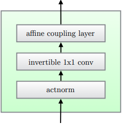
Glow

Glow^[9]

• Activation norm
• Invertible 1x1 convolution
• Affine coupling layers

Flow++

Flow++^[10]

• Dequantization via VI
• Improved coupling layers
  • Apply CDF for a mixture of $K$ logistics
  • stacking conv and multi-head self-attention

References

---

1. 1.Dinh, L., Krueger, D., & Bengio, Y. (2014). NICE: Non-linear Independent Components Estimation. CoRR, abs/1410.8516. ↩
2. 2.Dinh, L., Sohl-Dickstein, J., & Bengio, S. (2016). Density estimation using Real NVP. ArXiv, abs/1605.08803. ↩
3. 3.CS294-158 Lecture 2c+3a slides ↩
4. 4.CS228 notes: sampling methods ↩
5. 5.Rezende, D.J., & Mohamed, S. (2015). Variational Inference with Normalizing Flows. ArXiv, abs/1505.05770. ↩
6. 6.Chen, X., Kingma, D.P., Salimans, T., Duan, Y., Dhariwal, P., Schulman, J., Sutskever, I., & Abbeel, P. (2016). Variational Lossy Autoencoder. ArXiv, abs/1611.02731. ↩
7. 7.Papamakarios, G., Murray, I., & Pavlakou, T. (2017). Masked Autoregressive Flow for Density Estimation. NIPS. ↩
8. 8.Kingma, D.P., Salimans, T., & Welling, M. (2017). Improved Variational Inference with Inverse Autoregressive Flow. ArXiv, abs/1606.04934. ↩
9. 9.Kingma, D.P., & Dhariwal, P. (2018). Glow: Generative Flow with Invertible 1x1 Convolutions. NeurIPS. ↩
10. 10.Ho, J., Chen, X., Srinivas, A., Duan, Y., & Abbeel, P. (2019). Flow++: Improving Flow-Based Generative Models with Variational Dequantization and Architecture Design. ICML. ↩
11. 11.Müller, T., McWilliams, B., Rousselle, F., Gross, M., & Novák, J. (2018). Neural Importance Sampling. ACM Trans. Graph., 38, 145:1-145:19. ↩
12. 12.Grathwohl, W., Chen, R.T., Bettencourt, J., Sutskever, I., & Duvenaud, D. (2018). FFJORD: Free-form Continuous Dynamics for Scalable Reversible Generative Models. ArXiv, abs/1810.01367. ↩
13. 13.Huang, C., Krueger, D., Lacoste, A., & Courville, A.C. (2018). Neural Autoregressive Flows. ArXiv, abs/1804.00779. ↩
14. 14.Oord, A.V., Li, Y., Babuschkin, I., Simonyan, K., Vinyals, O., Kavukcuoglu, K., Driessche, G.V., Lockhart, E., Cobo, L.C., Stimberg, F., Casagrande, N., Grewe, D., Noury, S., Dieleman, S., Elsen, E., Kalchbrenner, N., Zen, H., Graves, A., King, H., Walters, T., Belov, D., & Hassabis, D. (2017). Parallel WaveNet: Fast High-Fidelity Speech Synthesis. ArXiv, abs/1711.10433. ↩