Likelihood-based Generative Models I: Autoregressive Models

The brain has about 10¹⁴ synapses and we only live for about 10⁹ seconds. So we have a lot more parameters than data. This motivates the idea that we must do a lot of unsupervised learning since the perceptual input (including proprioception) is the only place we can get 10⁵ dimensions of constraint per second.
(Geoffrey Hinton)

Unsupervised learning can be used to capture rich patterns in raw data with deep networks in a label-free way.

• Generative models: recreate raw data distribution
• Goal: learn some underlying hidden structure of the data
• Self-supervised learning: “puzzle” tasks that require semantic understanding to improve downstream tasks.
• Examples: clustering , dimensionality reduction, compression, feature learning, density estimation

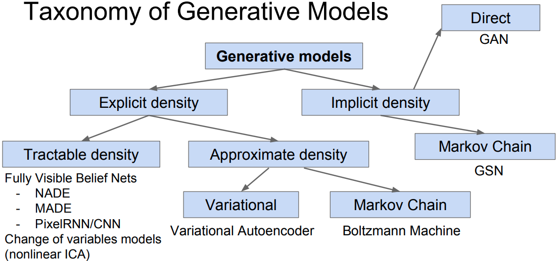
Main generative models:

• Autoregressive
• Normalizing flow
• Variational Autoencoder
• Generative Adversarial Networks

Real applications:

• generating data: synthesizing images, videos, speech, texts
• compressing data: constructing efficient codes
• anomaly detection

Image source: ^[20]

Likelihood-based models:

• estimate $p_\text{data}$ from samples $x^{(1)},\cdots,x^{(n)} \sim p_\text{data}(x)$

Given a dataset $\mathbf{x}^{(1)},\cdots,\mathbf{x}^{(n)}$, find $\theta$ by solving the optimization problem:

$$\arg\min_\theta J(\theta,\mathbf{x}^{(1)},\cdots,\mathbf{x}^{(n)}) = \frac{1}{n}\sum_{i=1}^n - \log p_\theta (\mathbf{x}^{(i)})$$

which is equivalent to minimizing KL divergence between the empirical data distribution and the model:

$$\begin{align} \hat{p}_\text{data}(\mathbf{x}) &= \frac{1}{n} \sum_{i=1}^n \mathbb{I}[\mathbf{x}=\mathbf{x}^{(i)}] \\ \mathbb{KL}(\hat{p}_\text{data} \| p_\theta) &= \mathbb{E}_{\mathbb{x}\sim \hat{p}_\text{data}} [- \log p_\theta(\mathbf{x})] - \mathbb{H}(\hat{p}_\text{data}) \end{align}$$

• MLE + SGD
• p_$\theta$ $\rightarrow$ NN

Autoregressive models

Autoregressive (AR) models share parameters among conditional distributions:

1. RNNs
2. Masking convolutions & attentions

The AR property is that each output $x_d$ only dependes on the previous input units $\mathbf{x}_{<d}$, but not on the future:

$$p(\mathbf{x}) = \prod_{d=1}^D p(x_d \vert \mathbf{x}_{<d})$$

AR models can only model discrete data.

RNN AR models

RNNs privode a compact, shared parameterization of a sequence of conditional distributions, shown to excel in handwriting generation, character prediction, machine translation, etc.

RNN LM

Given sequence of characters $\mathbf{x}$, $i$ indicates the position of characters:

$$\log p(\mathbf{x}) = \sum_{i=1}^d \log p(x_i \vert \mathbf{x}_{1:i-1})$$

Raw LSTM layers:

$$\begin{align} \left[\begin{array}{c} \mathbf{i}^c_j\\ \mathbf{o}^c_j \\ \mathbf{f}^c_j \\ \tilde{c}^c_j \end{array}\right] &= \left[\begin{array}{c} \sigma \\ \sigma \\ \sigma \\ \tanh \end{array}\right] (\mathbf{W}^{c^T} \left[\begin{array}{c} \mathbf{x}^c_j \\ \mathbf{h}^c_{j-1}\end{array}\right] + \mathbf{b}^c) \\ \mathbf{c}^c_j &= \mathbf{f}^c_j \odot \mathbf{c}^c_{j-1} + \mathbf{i}^c_j \odot \tilde{c}^c_{j} \\ \mathbf{h}_j^c &= \mathbf{o}_j^c \odot \tanh(\mathbf{c}^c_j) \end{align}$$

PixelRNN

Like in LM, AR models cast the joint distribution of pixels in the images to a product of conditional distributions, turning the joint modeling problem into a sequential problem with factorization, where one learns to predict the next pixel given all preivous generated pixels.

PixelRNN leverages two-dimensional RNNs and residual connections^[1] in generative image modeling.

Pixel-by-pixel generation

The probability $p(\mathbf{x})$ to each image $\mathbf{x}$ of $n \times n$ pixels. The image $\mathbf{x}$ is tiled as 1-D sequence $x_1, \cdots, x_{n^2}$ where pixels are taken from the image row by row. The joint distribution $p(\mathbf{x})$ is the product of the conditional probability over pixels:

$$p(\mathbf{x}) = \prod_{i=1}^{n^2} p(x_i \vert x_1, \cdots, x_{i-1})$$

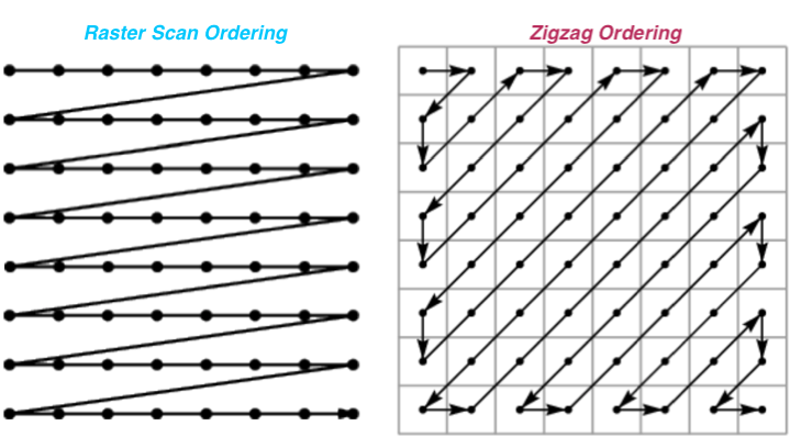
where each pixel is conditioned on all the previous generated pixels, whose generation is in the raster scan order: row by row and pixel by pixel within each row.

Taking into account RGB color channels of each pixel, the distribution of pixel $x_i$ is:

$$p(x_i \vert \mathbf{x}_{<i}) = p(\color{red}{x_{i,R}} \vert \mathbf{x}_{<i}) p(\color{green}{x_{i,G}} \vert \mathbf{x}_{<i}, \color{red}{x_{i,R}}) p(\color{blue}{x_{i, B}} \vert \mathbf{x}_{<i}, \color{red}{x_{i, R}}, \color{green}{x_{i, G}})$$

PixelRNN employs the discrete distribution with a 256-way softmax. Each channel variable $x_{x,*}$ takes the scalar values from 0 to 255. The advantages:

1. to be arbitrarily multimodal without prior on the shape;
2. achieve better results than continuous distribution and easy to learn.

• Training & evaluation -> the pixel distribution is parallel distribution (teacher forcing)
• Generation -> sequential, row by row and pixel by pixel.

Image source: PixelRNN^[1]

Row LSTM

Row LSTM is a unidirectional LSTM layer that takes the image row by row from top down to bottom computing features with 1-D convolution for a whole row at once.

It captures a roughly “triangular context” above the pixel with kernel size of $k \times 1$ in temporal convolutions where $k \leq 3$, of which the larger kernel size captures the broader contexts and weight sharing guarantees the translation invariance.

• Row LSTMs have the triangular receptive field, unable capturing the entire available context.

The computation proceeds as follows.

• LSTM layers have an input-to-state (is) and recurrent state-to-state (ss) component that together determine the four gates inside the LSTM core.
• The input-to-state component is precomputed using 1-D masked convolution with kernel size $k \times 1$ horizontally, where $\{ \mathbf{i}^c_j, \mathbf{o}^c_j, \mathbf{f}^c_j, \tilde{c}^c_j\} \in \mathbb{R}^{h \times n \times n}$, $h$ denotes the # of output feature maps.
• The row-wise state-to-state component of the LSTM layer takes the previous hidden and cell state $\mathbf{h}_{j-1}^c$ and $\mathbf{c}_{j-1}^c$, where $\{\mathbf{x}_i, \mathbf{h}_{j-1}^c, \mathbf{c}_{j-1}^c\} \in \mathbb{R}^{h \times n \times 1}$, the weights $\mathbf{K}^{ss}$ and $\mathbf{K}^{is}$ represent the kernel weights of state-to-state and input-to-state components, $\circledast$ denotes the convolution operation.

$$\begin{align} \left[\begin{array}{c} \mathbf{i}^c_j\\ \mathbf{o}^c_j \\ \mathbf{f}^c_j \\ \tilde{c}^c_j \end{array}\right] &= \left[\begin{array}{c} \sigma \\ \sigma \\ \sigma \\ \tanh \end{array}\right] ( \color{red}{ \mathbf{K}^\text{ss} \circledast \mathbf{h}_{j-1}^c} \color{blue}{+} \color{red}{ \mathbf{K}^\text{is} \circledast \mathbf{x}_{j} }) \\ \mathbf{c}^c_j &= \mathbf{f}^c_j \odot \mathbf{c}^c_{j-1} + \mathbf{i}^c_j \odot \tilde{c}^c_{j} \\ \mathbf{h}_j^c &= \mathbf{o}_j^c \odot \tanh(\mathbf{c}^c_j) \end{align}$$

Diagonal BiLSTM

Diagonal BiLSTM is designed to impede the drawbacks of limited triangular receptive fields of Row LSTM and could capture the entire available context.

Diagonal BiLSTM skews the input $\mathbf{x} \in \mathbb{R}^{n \times n}$ into $\mathbb{R}^{n \times (2n-1)}$ by shifting the $i$-th row with $(i-1)$ position offsets, i.e. each row is one position right shift compared with the previous row (see below figure).

• The input-to-state components of each direction adopt a $1 \times 1$ convolution $K^\text{is}$, and the output of $(\mathbf{K}^\text{is} \circledast \mathbf{x}) \in \mathbb{R}^{4h \times n \times n}$
• The state-to-state recurrent component uses a column-wise 1D convolution $K^\text{ss}$ with kernel size $2 \times 1$.
  Why 2x1? Larger sizes do not broaden the already global receptive fields.
• For bi-LSTMs, the right-to-left directional LSTM is shifted down by one row and added to the left-to-right LSTM outputs.

• Train the pixelRNN of up to 12 layers of depth with residual connections and layer-to-output skip connections.

Image source: ^[1]

Masking-based AR models

Key property: parallelized computation of all conditions

1. Masked MLP (MADE)
2. Masked convolutions & self-attention (PixelCNN families and PixelSNAIL)
   • also share parameters across time

MADE

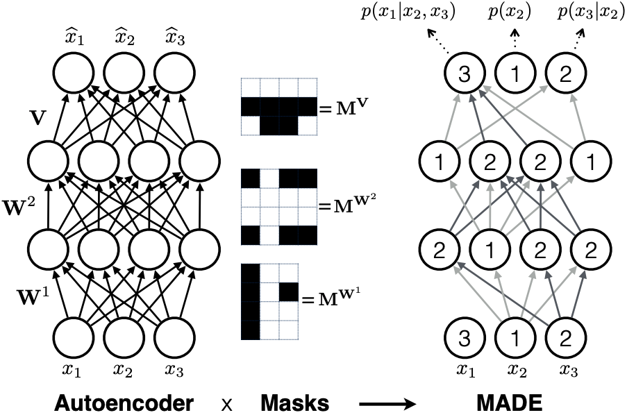
Masked Autoencoder Distribution Estimator (MADE) (Deepmind & Iain Murray)^[3] masks the autoencoder’s parameters to respect autoregressive properties that each input only reconstructed from previous input in a given ordering.

MADE zeros out the connections of layer connections by elementwise-multiplying a binary mask matrix on the weight matrices, setting the weight connectivities as 0s for removing.

For masked autoencoder with $L>1$ hidden layers, let

• $D$ denote the dimension of input $\mathbf{x}$, $\mathbf{M}$ denote the connection mask;
• in $l$-th layer, $K^l$ be the # of hidden states, $m^l(k)$ represent the maximum number of connected input of the $k$-th unit.

For $l$-th layer in masked autoencoders, the mask of weight matrices $\mathbf{W}$:

$$\mathbf{M}_{k^\prime, k}^{\mathbf{W}^l} = \mathbf{1}_{m^l(k^\prime) \leq m^{l-1}(k)} = \left\{ \begin{array}{ll} 1 & \text{if} \; m^l(k^\prime) \leq m^{l-1}(k) \\ 0 & \text{otherwise} \end{array} \right.$$

For the output mask of weight matrices $\mathbf{V}$:

$$\mathbf{M}_{d, k}^{\mathbf{V}} = \mathbf{1}_{d > m^L(k)} = \left\{ \begin{array}{ll} 1 & \text{if} \; d > m^L(k) \\ 0 & \text{otherwise} \end{array} \right.$$

Image source:^[3]

PixelCNN families

PixelCNN

PixelCNN^[1] adopts multiple conv layers without pooling to preserve the spatial resolution and masks the future context.

• Drawbacks: PixelRNNs cannot consider the pixels on the right side of the current position (as Fig. below).

Gated PixelCNN

Gated PixelCNN takes into account both the vertical stack and the horizontal stack by combing both the pixels of region above and those on the left of the current row, wherein the convolutions of vertical stack are not masked. (See ^[5] for the tutorial.)

• advantages: deal with “blind spot” of the receptive field in PixelCNNs.

Gated PixelCNNs replace the ReLU between masked convolutions in the original pixelCNN with the gated activation function:

$$\mathbf{y} = \tanh (w_{k,f} \circledast \mathbf{x}) \odot \sigma (W_{k,g} \circledast \mathbf{x})$$

where $p$ represents the # of feature maps, $\circledast$ denotes convolution operations, where it is masked in horizontal stack but unmasked in the vertical stack.

Conditional PixelCNN

Given high-level latent representation $\mathbf{h}$, we model the conditional PixelCNN models:

$$p(\mathbf{x} \vert \mathbf{h}) = \prod_{i=1}^{n^2} p(x_i \vert x_1, \cdots, x_{i-1}, \mathbf{h})$$

Add terms pf $\mathbf{h}$ before the non-linearities:

$$\mathbf{y} = \tanh (W_{k,f} \circledast \mathbf{x} \color{red}{+ V_{k,f}^\top \mathbf{h}} ) \odot \sigma (W_{k,g} \circledast \mathbf{x} \color{red}{+ V_{k,g}^\top \mathbf{h} })$$

where $k$ is the layer number.
Condition on what:

• class-dependent: $\mathbf{h} \rightarrow \text{1-hot}$, is equivalent to adding a class-dependent bias at each layer.

Condition on where:

• location-dependent: use Transposed convolution to map $\mathbf{h}$ to a spatial representation $\color{red}{\mathbf{s} = \text{deconv}(\mathbf{h})}$ to produce the output $\mathbf{s}$ of the same shape as the image. It can be seen as adding a location dependent bias: $$\mathbf{y} = \tanh (W_{k,f} \circledast \mathbf{x} \color{red}{+ V_{k,f} \circledast \mathbf{s}} ) \odot \sigma (W_{k,g} \circledast \mathbf{x} \color{red}{+ V_{k,g} \circledast \mathbf{s} })$$

PixelCNN++

Background:

• previous 256-way softmax is very costly and slow to compute, and makes the gradient w.r.t parameters very sparse.
• the model does not know that the value 128 is close to that of 127 and 129. Especially unobserved sub-pixels will be assigned with 0 probability.

PixelCNN++^[6] assumes the latent color intensity $\nu$ with continuous distribution and takes the continuous univariate distribution to be a mixture of logistic distributions.

• $\sigma(x) = -1 / (1+ \exp(- x))$.
• For all sub-pixels except the edges 0 and 255: $$\begin{align} \nu & \sim \sum_{i=1}^K \pi_i \text{logistic}(\mu_i, s_i) \\ P(x \vert \pi, \mu, s) &= \sum_{i=1}^K \pi_i [ \sigma \bigg( (\frac{x+0.5 - \mu_i}{s_i}) \bigg) - \sigma \bigg( (\frac{x-0.5 - \mu_i}{s_i}) \bigg) ] \end{align}$$
• For edge cases,
  1. when $x=0$, set $x-0.5 \rightarrow -\infty$
  2. when $x=255$, set $x+0.5 \rightarrow +\infty$

Logistic distribution:

$$\begin{align}F(x) &= \big(1+ e^{-\frac{x-\mu}{s}}\big)^{-1} \\&= \frac{1}{2} [1+\tanh (\frac{x-\mu}{2 s})]\end{align}$$

where the mean $ \mu \in (-\infty, +\infty)$, std deviation $s >0$

• PixelCNN++ does not use deep networks to model the relationship between color channels. For the pixel $(r_{i,j}, g_{i,j}, b_{i,j})$ at the location $(i,j)$ in the image, with the contexts $C_{i,j}$:

$$\begin{align} p(\color{red}{r}_{i,j}, \color{green}{g}_{i,j}, \color{blue}{b}_{i,j} \vert C_{i,j}) &= P \bigg(\color{red}{r}_{i,j} \vert \mu_\color{red}{r}(C_{i,j}), s_\color{red}{r}(C_{i,j})\bigg) \times P\bigg(\color{green}{g}_{i,j} \vert \mu_\color{green}{g} (C_{i,j}, \color{red}{r}_{i,j}), s_\color{green}{g}(C_{i,j})\bigg) \\ & \times P\bigg(\color{blue}{b}_{i,j} \vert \mu_\color{blue}{b} (C_{i,j}, \color{red}{r}_{i,j}, \color{green}{g}_{i,j}), s_\color{blue}{b}(C_{i,j}) \bigg) \\ \mu_\color{green}{g}(C_{i,j}, \color{red}{r}_{i,j}) &= \mu_\color{green}{g}(C_{i,j}) + \alpha(C_{i,j})\color{red}{r}_{i,j} \\ \mu_\color{blue}{b}(C_{i,j}, \color{red}{r}_{i,j}, \color{green}{g}_{i,j}) &= \mu_\color{blue}{b}(C_{i,j}) + \beta (C_{i,j}) \color{red}{r}_{i,j} + \gamma (C_{i,j}) \color{blue}{b}_{i,j} \end{align}$$

where $\alpha$, $\gamma$, $\beta$ are scalar coefficents depdenting on the mixture component and previous pixels.

• As shown in the figure, it applies convolutions of stride 2 for downsampling and transposed strided convolution for upsampling. It also uses shor-cut connections recover the information loss from convolutions in the lower layers, similar to VAE^[8] and U-Net^[7].

WaveNet

• Masked convolutions: masked convolution has limited receptive field and thus requires deep stacked layers of a linearly increased number. It requires expand the kernel size or incease the layer depth to enlarge the effective receptive fields. (see below figure)

WaveNet^[11][12] (van den Ood et al., DeepMind 2016) leverages dilated masked casual convolution to exponentially increase the receptive field. It is applied in TTS, ASR, music generation, audio modeling, etc.

Model architecture

It uses the same gated activation unit in PixelCNN, outperforming ReLU:

$$\mathbf{z} = \tanh (W_{f,k} \circledast \mathbf{x}) \odot \sigma(W_{g,k} \circledast \mathbf{x})$$

The overall model structure is: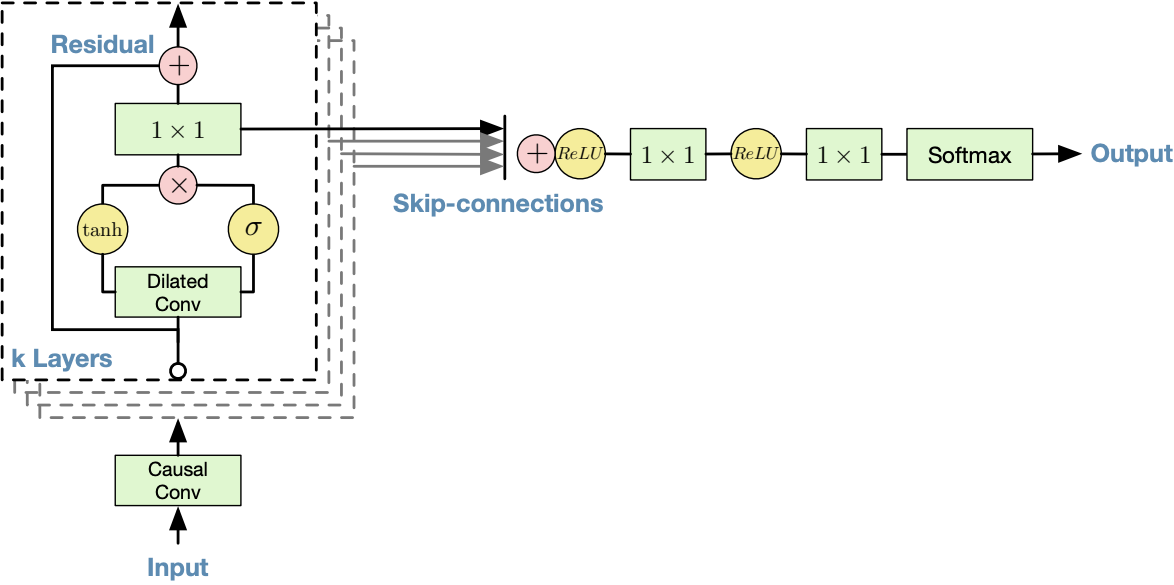

Conditional WaveNet

Like the conditional Gated PixelCNN, WaveNet can be also conditional on a hidden representation $\mathbf{h}$.

• Global conditioning on a single representation vector $\mathbf{h}$ that influences the output distribution of all timesteps, e.g. a speaker embedding in a TTS model: $$\mathbf{z} = \tanh (W_{f,k} \circledast \mathbf{x} + \color{red}{V_{f,k}^\top \mathbf{h}}) \odot \sigma(W_{g,k} \circledast \mathbf{x} + \color{red}{V_{g,k}^\top \mathbf{h}})$$
• Local conditioning on a second timeseries $h_t$, possibly with a lower sampling frequency than the audio, e.g. linguistic features in a TTS model. WaveNet learns the upsampling on this time series using a transposed convolution: $\mathbf{y} = f(\mathbf{h})$ $$\mathbf{z} = \tanh (W_{f,k} \circledast \mathbf{x} + \color{red}{V_{f,k} \circledast f(\mathbf{h})}) \odot \sigma(W_{g,k} \circledast \mathbf{x} + \color{red}{V_{g,k} \circledast f(\mathbf{h})})$$

Softmax distribution

The raw audio output is stored as a sequence of 16-bit scalar values (one per time step), thus the softmax output is 2¹⁶=65,536 probabilities per timestep. WaveNet applies a $\mu$-law companding transformation to the data and thenquantize it to 256 possible values:

$$f(x_t) = \text{sign} (x_t) \frac{\ln(1 + \mu |x_t|)}{\ln(1 + \mu)}$$

where $x_t \in (-1,1)$, $u=255$. The reconstruction signal after quantization sounded similar to the original.

Fast generation via caching

Problems: During generation, convolutional AR models redundantly compute states, impeding the speed of generation process. Such states can be cached and reused to expedite the generation.^[14]

The convolutional autoregressive generative model could cache and reuse the previously computed hidden states to accelerate the generation.

The below figure shows the model with 2 convolutional and 2 transposed convolutional layers with strid of 2, wherein blue dots indicate the cached states and orange bots are computed in the current step. The computation process can be seen as:

Image source: ^[14]

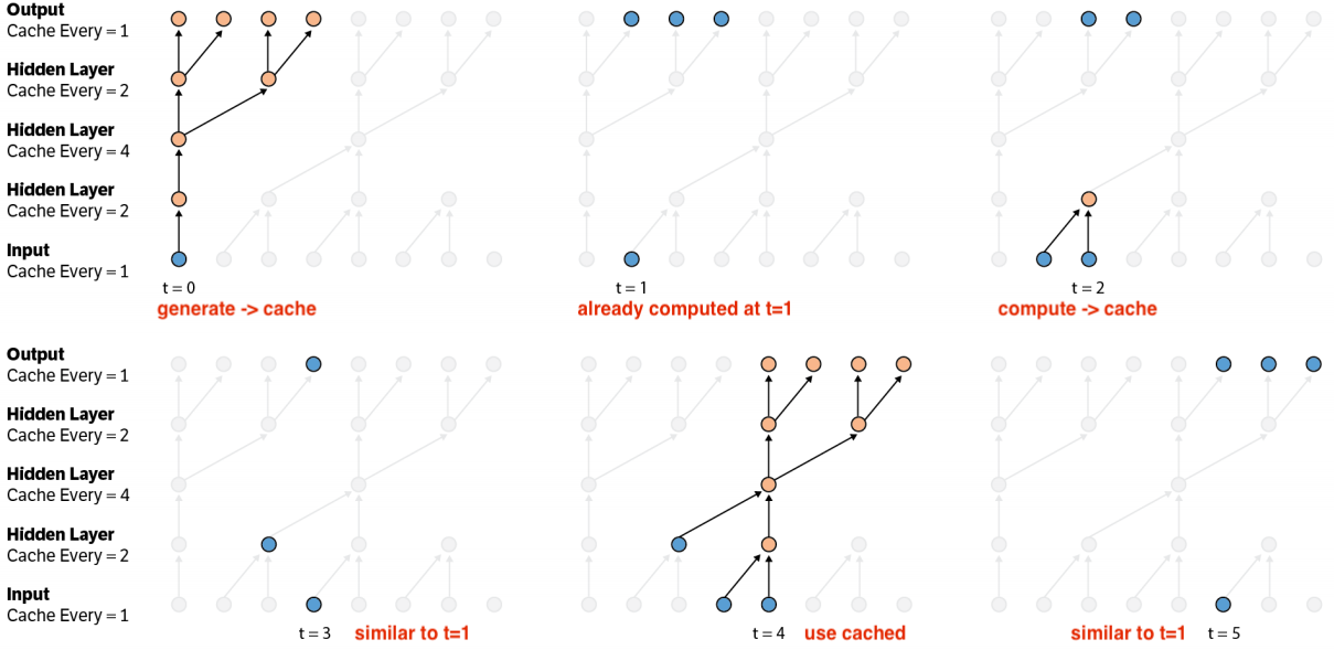
• This can also scale to 2D to apply on PixelCNN families^[14].

PixelSNAIL

PixelSNAIL^[10] adopt masked self-attention approaches inspired by SNAIL^[9].

Model architecture

The overall model structure:

• It uses the self-attention block with shape $H \times W \times C_1 \rightarrow H \times W \times C_2$ (see below figure):

  • Key f_k: $C_1 \rightarrow \text{d}_\text{key}$
  • Query f_q: $C_1 \rightarrow \text{d}_\text{key}$

  • Value f_v(x): $C_1 \rightarrow C_2$

    Given 2D feature map $\mathbf{y}= {y_1, y_2, \cdots, y_N }$, the attention mapping is:

    $$\begin{align} z_i & = \sum_{j<i} e_{ij} f_v(y_i) \\ e_i &= \text{softmax}([f_k(y_1)^\top f_q(y_i), \cdots, f_k(y_i-1)^\top f_q(y_i)]) \end{align}$$

    where the summation over all previous history, i.e. $j<i$.

• It applies 2D convolutions with gated activation functions as gated &PixelCNN* and residual connections as the figure.

• It adopts the zigzag ordering rather than PixelCNN-like raster scan ordering.

• It employs the discretized mixture of logistics of PixelCNN++ as the output distribution.

In comparison,

• Gated PixelCNN and PixelCNN++ apply causal convolutions (dilated and strided conv, respectively) over the sequence, allowing the high-brandwidth access to the previous pixels. However, caual convolutions are limited to the receptive field due to their finite sizes.
• PixelSNAIL achieves a much larger receptive field size (see below figure).

Analysis

“The basic difference between AR models with Generative Adversarial Networks (GANs) is that GANs implicitly learn data distribution whereas AR models learn the explicit distribution governed by a prior. “^[15]

Pros:

• expressivity (explicit learn): AR factorization is general; can explicitly compute likelihood $p(x)$
• explicit likelihood of training data gives good evaluation metric
• good samples
• generalization: meaningful parameter sharing has good inductive bias
• the training is more stable than GANs
• it works for both discrete and continuous data (It is hard to learn discrete data like text for GANs)

Cons:

• Sequential generation => slow!
• Low sampling efficency: sampling each pixel = 1 forward pass!

Reference

---

1. 1.Oord, A. V. D., Kalchbrenner, N., & Kavukcuoglu, K. (2016). Pixel recurrent neural networks. (Google DeepMind). ICML 2016. ↩
2. 2.The Unreasonable Effectiveness of Recurrent Neural Networks. Andrej Karpathy blog ↩
3. 3.Germain, M., Gregor, K., Murray, I., & Larochelle, H. (2015, June). Made: Masked autoencoder for distribution estimation. In International Conference on Machine Learning (pp. 881-889). ↩
4. 4.Van den Oord, A., Kalchbrenner, N., Espeholt, L., Vinyals, O., & Graves, A. (2016). Conditional image generation with pixelcnn decoders. In Advances in neural information processing systems (pp. 4790-4798). ↩
5. 5.Tutorial: Gated PixelCNN ↩
6. 6.Salimans, T., Karpathy, A., Chen, X., & Kingma, D. P. (2017). Pixelcnn++: Improving the pixelcnn with discretized logistic mixture likelihood and other modifications. arXiv preprint arXiv:1701.05517. ↩
7. 7.Ronneberger, O., Fischer, P., & Brox, T. (2015, October). U-net: Convolutional networks for biomedical image segmentation%E5%92%8CTiramisu. In International Conference on Medical image computing and computer-assisted intervention (pp. 234-241). Springer, Cham. ↩
8. 8.Kingma, D. P., Salimans, T., Jozefowicz, R., Chen, X., Sutskever, I., & Welling, M. (2016). Improved variational inference with inverse autoregressive flow. In Advances in neural information processing systems (pp. 4743-4751). ↩
9. 9.Mishra, N., Rohaninejad, M., Chen, X., & Abbeel, P. (2017). A simple neural attentive meta-learner. arXiv preprint arXiv:1707.03141. ↩
10. 10.Chen, X., Mishra, N., Rohaninejad, M., & Abbeel, P. (2017). Pixelsnail: An improved autoregressive generative model. ICML 2018. ↩
11. 11.Oord, A. V. D., Dieleman, S., Zen, H., Simonyan, K., Vinyals, O., Graves, A., ... & Kavukcuoglu, K. (2016). Wavenet: A generative model for raw audio. arXiv preprint arXiv:1609.03499. ↩
12. 12.(DeepMind blog) WaveNet: A generative model for raw audio ↩
13. 14.Ramachandran, P., Paine, T. L., Khorrami, P., Babaeizadeh, M., Chang, S., Zhang, Y., ... & Huang, T. S. (2017). Fast generation for convolutional autoregressive models. arXiv preprint arXiv:1704.06001. ↩
14. 15.(TowardsDataScience blog) Auto-Regressive Generative Models (PixelRNN, PixelCNN++) [^16:] CS294-158 Lecture 2 slides ↩
15. 17.Parallel Multiscale Autoregressive Density Estimation ↩
16. 18.PixelCNN Models with Auxiliary Variables for Natural Image Modeling ↩
17. 19.GENERATING HIGH FIDELITY IMAGES WITH SUBSCALE PIXEL NETWORKS AND MULTIDIMENSIONAL UPSCALING ↩
18. 20.Stanford cs231n: Generative models ↩