Go Deeper in Convolutions: a Peek

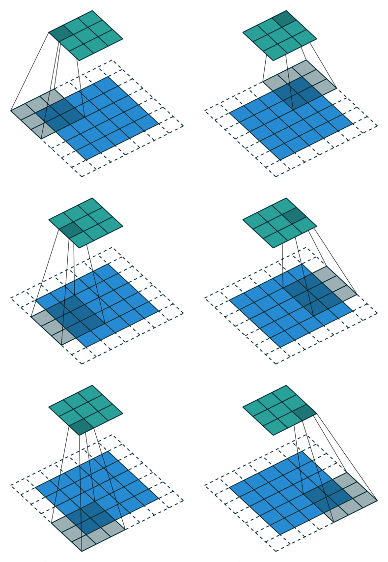
The main aim of conv op is to extract useful features for downstream tasks. And different filters could intuitionally extract different aspect of features via backprop during training. Afterward, all the extracted features are combined to make decisions.

Convolutional Networks

ConvNets including local receptive fields, weight sharing, and pooling, leading to:

1. Modeling the spatial structure
2. Translation invariance
3. Local feature detection

Standard discrete convolution:

$$(f*k)(\mathbf{p}) = \sum_{s+t=p}F(s)k(t)$$

• channels == feature maps.
• channels are used to describe the structure of a layer, while the kernel is used to describe the structure of a filter.^[5]
• A “kernel” refers to a 2D array of weights, while a “filter” refers to a 3D structure of multiple kernels stacked together. In 2D filters, filter==kernel; in 3D filters, a filter -> a collection of stacked kernels.
• Each filter provides one output channel.

Properties

• Weights (i.e. the conv kernel) are shared across all hidden states
• Spatial correspondence between pixels and hidden units (“2D matrix of hidden units”=”feature map”)
• Translation invariance: extract the same features irrespective of where an image patch is located in the input.

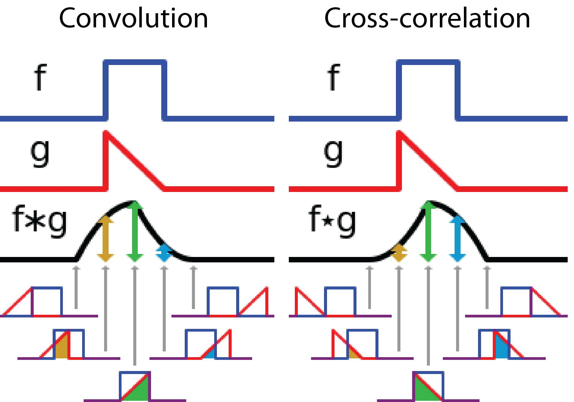
convolution v.s. cross-correlation

• Convolution in signal processing: $$(f * g)(t) = \int_{-\infty}^\infty f(\tau) g(t-\tau)d\tau$$ the filter $g$ is reversed and then slides along the axis.
• Cross-correlation is sliding non-reversed filter $g$ through the function $f$.

2D convolution

• Input: 4-dim tensor (N,$C_\text{in}$,H,W) -> (minibatch-size, num-featuremaps, x, y)
• Filters: 4-dim tensor ($C_\text{out}$, $C_\text{in}$, kernel_dim1, kernel_dim2)
• Output: 4-dim tensor (N, $C_\text{out}$, output_dim1, output_dim2)

2D-convolution op sums all the element-wise convolution results along $c_\text{in}$ axis -> squeeze the $c_\text{in}$ axis to 1 by sum op.

Conv layer

The filter depth is the same as the input layer depth.^[5] We can intuitionally think multi-channel conv op as sliding a 3D filter matrix through the input layer, performing element-wise multiplication and addition, where the 3D filter moves only in 2-direction,i.e. height and width of the image.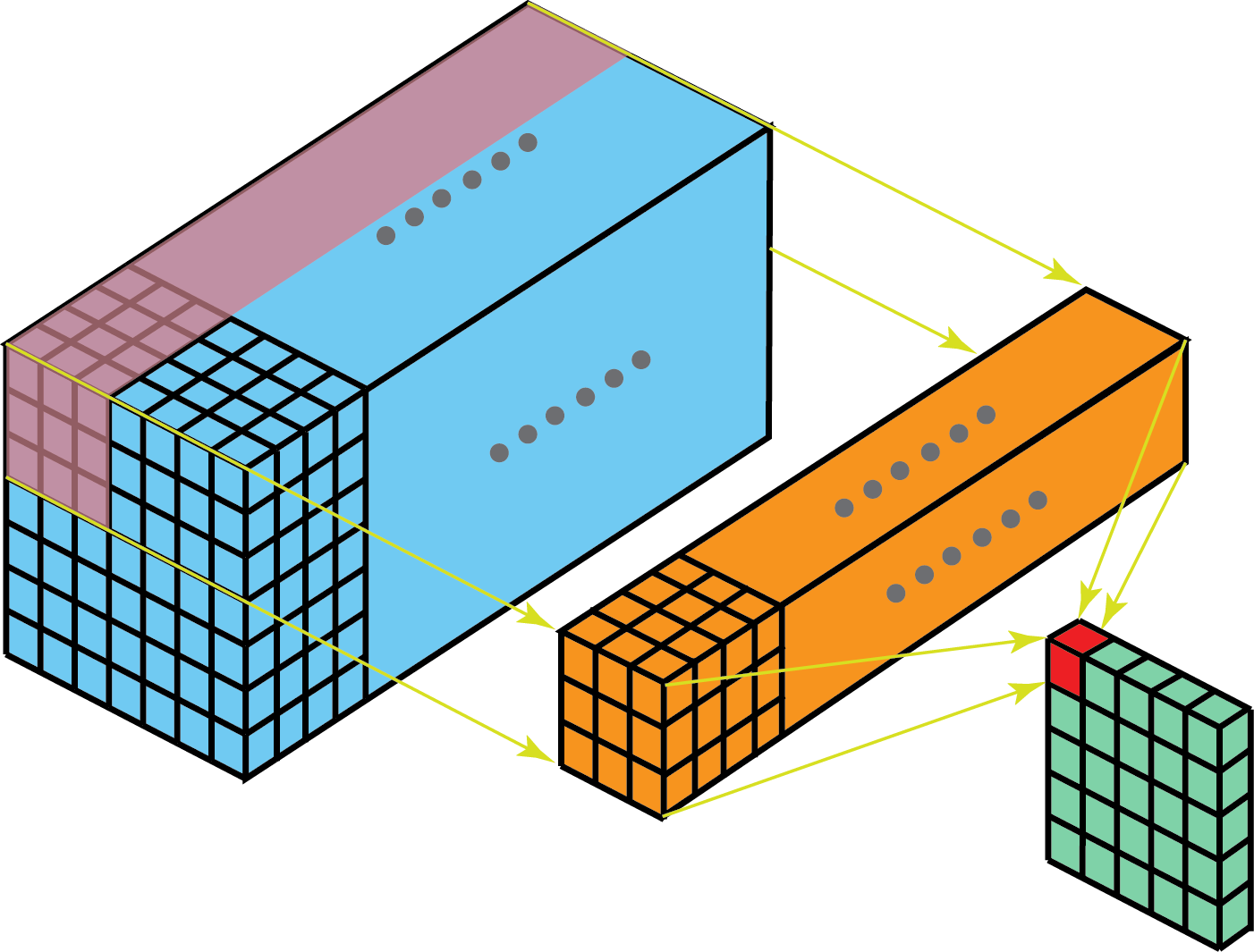

• Input size: $W_1 \times H_1 \times D_1$
• Requires 4 hyperparams:
  1. # of filters $K$
  2. filter size $F$
  3. stride $S$
  4. padding size $P$
• Output size $W_2 \times H_2 \times D_2$
  1. $W_2 = \text{lower_bound}\frac{W_1 + 2P -F}{S} + 1$
  2. $H_2 = \text{lower_bound}\frac{H_1 + 2P-F}{S} + 1$
  3. $D_2 = K$
• # of parameters $$\underbrace{F \cdot F \cdot D_1 \cdot K}_\text{ # of weight params} + \underbrace{K}_\text{ # of biases}$$

Time complexity of conv op

The time complexity of single Conv layer:

$$O( \underbrace{ \text{(out-feature-map-size)}^2 }_\text{the area of output feature map} \cdot \underbrace{\text{(Kernel-size)}^2}_\text{area of single kernel} \cdot C_\text{in} \cdot C_\text{out} )$$

• where $C_\text{in}$ and $C_\text{out}$ denote the # of output channel.

Total time complexity of all conv layers (sum over all the conv layers):

$$O \big(\sum_{l=1}^D \underbrace{ \text{(out-feature-map-size)}_l^2 }_\text{the area of output feature map} \cdot \underbrace{\text{(Kernel-size)}_l^2}_\text{area of single kernel} \cdot C_{l-1} \cdot C_l \big)$$

where

• $D$ is the depth of conv layers
• $C_{l-1}$ means the input channel # of current layer, i.e. the output channel # of previous layer.

Space complexity of conv op

The space complexity includes the # of weights and the size of output feature map.

$$O(\sum_{l=1}^D \text{(kernel-size)}^2_l \cdot C_{l-1} \cdot C_l + \sum_{l-1}^D \text{(feature-map-size)}^2 \cdot C_l )$$

Pooling layer

• Input size $W_1 \times H_1 \times D_1$
• Requires 2 hyperparams:
  1. pooling size $F$
  2. stride size $S$
• Output size $W_2 \times H_2 \times D_2$:
  1. $W_2 = (W_1-F)/S + 1$
  2. $H_2 = (H_1-F)/S +1$
  3. $D_2 = D_1$
• Zero parameters since it computes a fixed function
• Discarding pooling layers has shown to be imortant in training good generative models, e.g, VAEs and GANs ^[1]

Conv implementation

im2col

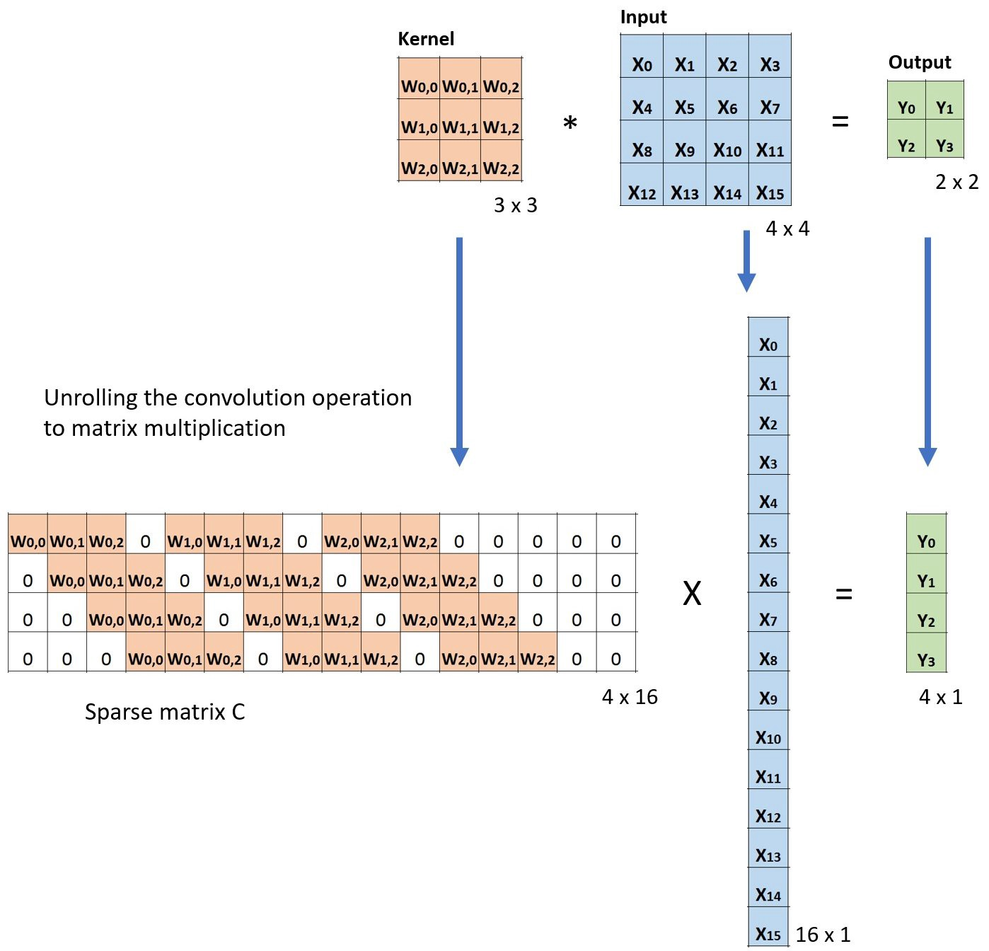
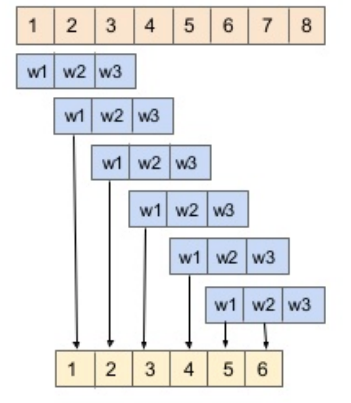
1D convolution

Convolve along one axis (i.e. the sequential direction in NLP), with the kernel width the same as the input length, which is commonly used in TextCNNs. The kernel width $L_\text{in}$ is the same as the input width, i.e. the size of embedding.

The shape of dilated conv2d:

• Input $(N, C_\text{in}, L_\text{in})$
• Output: $(N, C_\text{out}, L_\text{out})$

$$L_\text{out}=\lfloor \frac{L_\text{in} + 2 \times \text{padding} - \text{dilation} \times (\text{kernel_size} -1) -1 }{\text{stride}} + 1 \rfloor$$

1x1 convolution

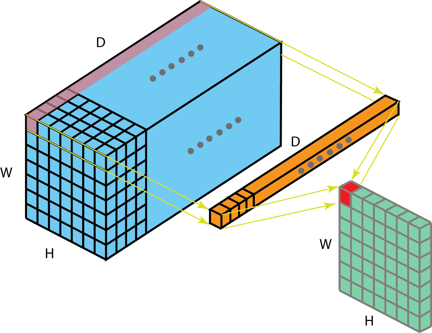
$1 \times 1$ convolution is proposed in Network in Network (NIN)^[6]. It can be used for:

• dimensionality reduction for efficient computations
• efficient low dimensional embedding, or feature pooling
• applying non-linearity again after convolution.

$1 \times 1$ convolution can be used to reduce the dimension depth-wise.

Transposed convolution(Deconvolution)

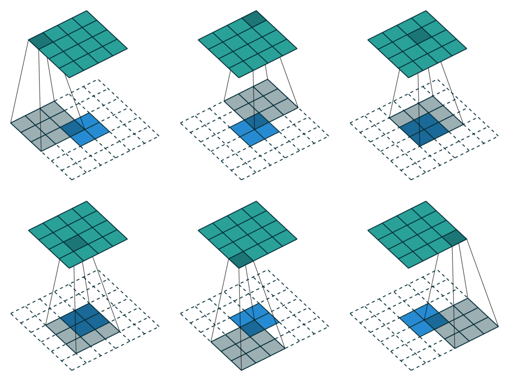
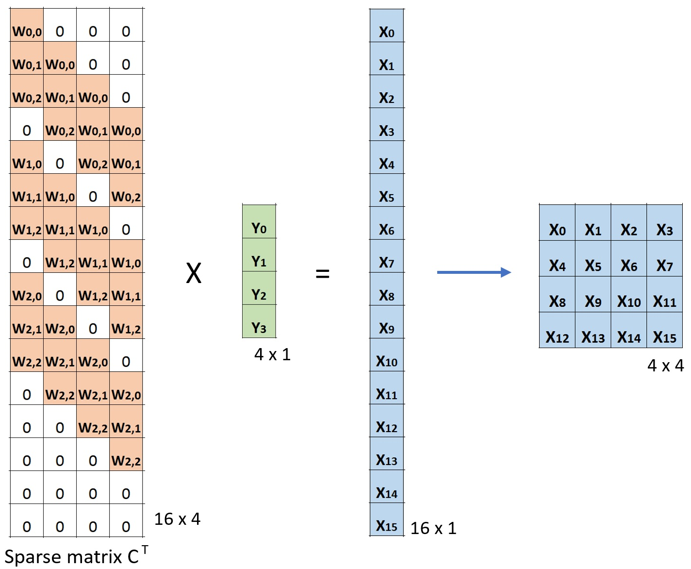
Transposed convolution (a.k.a deconvolution, fractionally strided convolution) is used to perform up-sampling, i.e. doing transformations in the opposite direction of a normal convolution.
It can be used in:

• generating high-resolution images
• mapping a low dimensional feature map to high dimensional space

• Input dim $(N, C_\text{in}, H_\text{in}, W_\text{in})$
• output dim $(N, C_\text{out}, H_\text{out}, W_\text{out})$
  where the dim: $$H_\text{out} = \text{stride}[0] \times (H_\text{in}-1) - 2 \times \text{padding}[0] + \text{dilation}[0] \times (\text{kernel[0] - 1}) + \text{out_pad[0]} + 1$$ $$W_\text{out} = \text{stride}[1] \times (W_\text{in}-1) - 2 \times \text{padding}[1] + \text{dilation}[1] \times (\text{kernel[1] - 1}) + \text{out_pad[1]} + 1$$

Transposed conv implementation

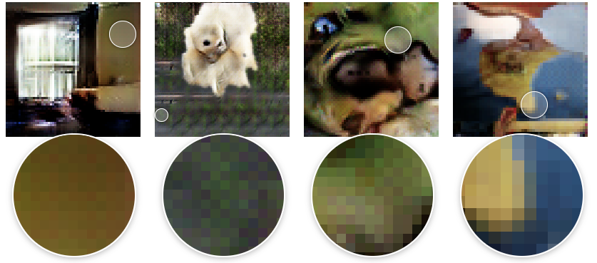
Checkerboard artifacts

Checkerboard artifacts result from “uneven overlap” pf transposed convolution^[8]. As shown in the following image, images on the bottom are the result of transposed convolution on the top row images. With transposed conv, a layer with a small size can be mapped to a layer with the larger size.

“The transposed convolution has uneven overlap when the filter size is not divisible by the stride. This “uneven overlap” puts more of the paint in some places than others, thus creates the checkerboard effects.”^[7]

Image source: ^[8]

Solution

1. Assure that the filter size can be divided by the stride, to avoid overlap issue
2. Use transposed Conv with stride = 1

A better up-sampling approach:

• resize the image first (using nearest-neighbor interpolation or bilinear interpolation) and then do a conv layer. -> avoid checkerboard effects

Dilated convolution (Atrous conv)

Dilated convolutions inflate the kernel by inserting spaces between the kernel elements, with usually l-1 spaces inserted between kernel elements.^[9]

With dilated conv, we can observe a large receptive field without increasing the kernel size, which is effective when stacking multiple dilated convolutions one after another.

$$(f*_l k)(\mathbf{p}) = \sum_{\mathbf{s}+l\mathbf{t}=\mathbf{p}}F(\mathbf{s})k(\mathbf{t})$$

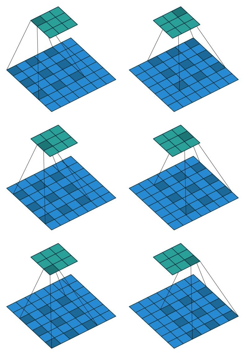
In PyTorch, dilation param means the space between kernel elements, with default 1.
Dilation =1 means no dilation.

The shape of dilated conv2d:

• Input $(N, C_\text{in}, H_\text{in}, W_\text{in})$
• Output: $(N, C_\text{out}, H_\text{out}, W_\text{out})$

$$H_\text{out}=\lfloor \frac{H_\text{in} + 2 \times \text{padding} - \text{dilation} \times (\text{kernel_size} -1) -1 }{\text{stride}} + 1 \rfloor$$ $$W_\text{out}=\lfloor \frac{W_\text{in} + 2 \times \text{padding} - \text{dilation} \times (\text{kernel_size} -1) -1 }{\text{stride}} + 1 \rfloor$$

Separable convolutions

Spatially separable convolutions

Spatially separable conv divides kernels into two vectors, and do convolution one by one.

• drawbacks: not all filters can be divided into two smaller kernels. The training result may be sub-optimal.

Depthwise separable convolutions

The depth-wise separable convolutions consist of two steps: depthwise convolutions and 1x1 convolutions. It is commonly used in MobileNet and Xception.

• Pros: efficient!

Grouped convolutions

Grouped convolutions are proposed by AlexNet paper. Filters are separated into different groups, each group is responsible for a conventional 2D convolutions with a certain depth.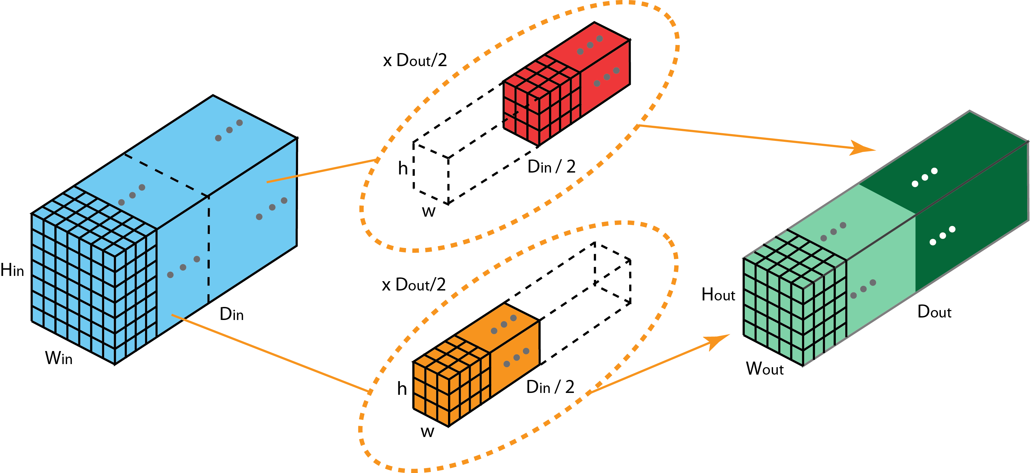

Variant convolutions

• Flattened Conv
• Shuffled Grouped Conv (ShuffleNet)
• Pointwise grouped Conv (ShuffleNet)

Inception

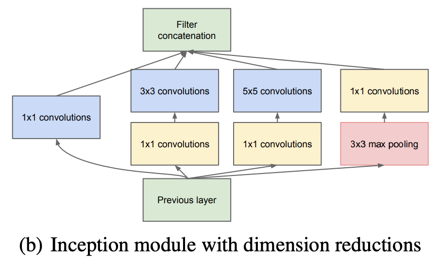
Inception module is designed to increase the depth and width of the network while keeping the computational cost constant.^[4]

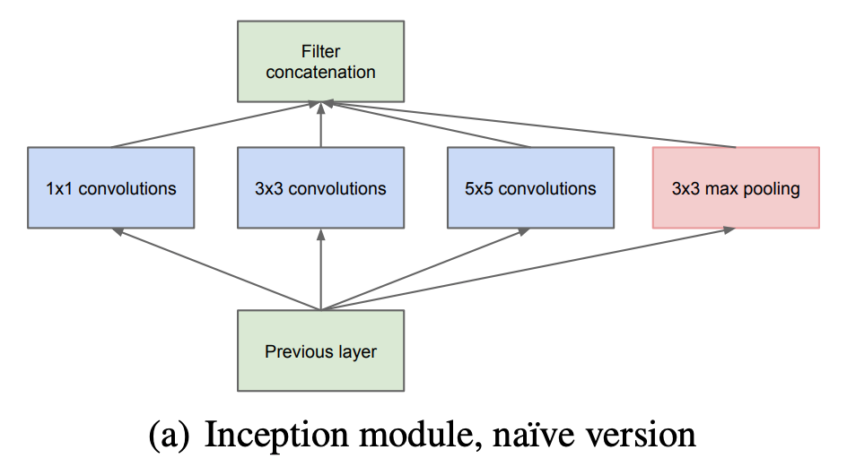
Inception modules apply 1x1 convolution to reduce dimensions before the expensive 3x3 and 5x5 convolutions. 1x1 can also include the use of rectified linear activation.

Pros:^[4]

• increase the # of units at each stage significantly without an uncontrolled blow-up in computational complexity
• Align with the intuition that, aggregate processed visual information at different scales could be useful, so that following stage can abstract features from different scales simultaneously.

ResNet

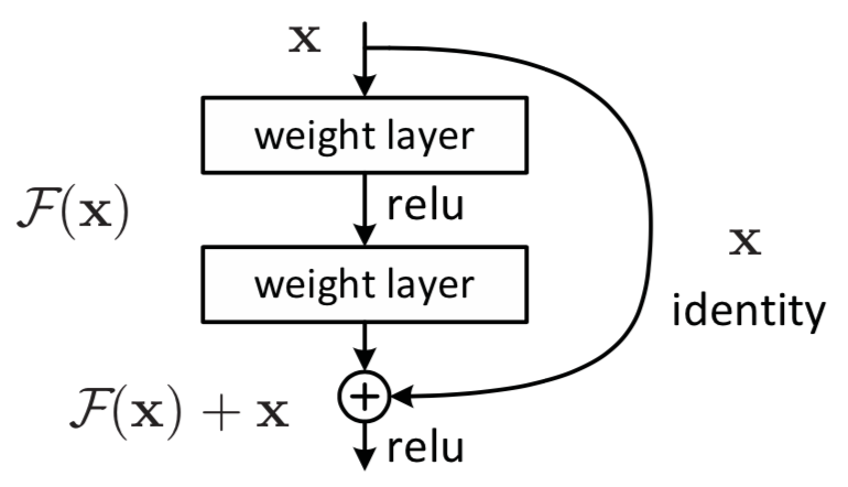
ResNet^[11] was proposed to explicitly fit a residual mapping. Instead of directly fitting the desired mapping as $\mathcal{H}(\pmb{x})$, use stacked non-linear layers to fit the residual mapping $\mathcal{F}(\pmb{x}):= \mathcal{H}(\pmb{x}) - \pmb{x}$. The original mapping is thus recast into $\mathcal{F}(\pmb{x})+\pmb{x}$.

• Intuitionally, to the extreme, if an identity mapping were optimal, pushing the residual to zero is much easier than to fit an identity mapping by a stack of non-linear layers.^[11]
• “+” shortcut connections introduce nor extra parameter neither computational complexity.

Image source:^[11]

ResNet vs Highway Nets

• “Highway nets” can be seen as a shortcut connection with gated functions, whose gates are data-dependent and have parameters to be trained.
• To the extreme, if the gate in Highway nets is closed (~0), the highway net is non-residual at all.

References

---

1. 1.http://cs231n.github.io/convolutional-networks/ ↩
2. 2.blog (in Chinese): complexity analysis of CNNs (in Chinese) ↩
3. 3.He, K., & Sun, J. (2015). Convolutional neural networks at constrained time cost. In Proceedings of the IEEE conference on computer vision and pattern recognition (pp. 5353-5360). ↩
4. 4.Szegedy, C., Liu, W., Jia, Y., Sermanet, P., Reed, S., Anguelov, D., ... & Rabinovich, A. (2015). Going deeper with convolutions. In Proceedings of the IEEE conference on computer vision and pattern recognition (pp. 1-9). ↩
5. 5.A Comprehensive Introduction to Different Types of Convolutions in Deep Learning ↩
6. 6.Lin, M., Chen, Q., & Yan, S. (2013). Network in network. arXiv preprint arXiv:1312.4400. ↩
7. 7.A guide to convolution arithmetic for deep learning ↩
8. 8.Deconvolution and Checkerboard Artifacts ↩
9. 9.Chen, L. C., Papandreou, G., Kokkinos, I., Murphy, K., & Yuille, A. L. (2014). Semantic image segmentation with deep convolutional nets and fully connected crfs. arXiv preprint arXiv:1412.7062. ↩
10. 10.Up-sampling with Transposed Convolution ↩
11. 11.He, K., Zhang, X., Ren, S., & Sun, J. (2016). Deep residual learning for image recognition. In Proceedings of the IEEE conference on computer vision and pattern recognition (pp. 770-778). ↩
12. 12.Dumoulin, V., & Visin, F. (2016). A guide to convolution arithmetic for deep learning. arXiv preprint arXiv:1603.07285. ↩
13. 13.Transposed CNN (in Chinese) ↩