Deep Q-Networks: A Summary

A summary of key advances of Deep Q-Networks.

Nature DQN (Nature 2015)

Challenge:

1. Sparse, noisy and delayed reward. The scalar reward signal is frequently sparse, noisy and delayed. The delay between actions and rewards can be thousands of time steps long.
2. Highly-correlated data. Deep learning assume the data samples to be independent, whilst in RL one typically encounters sequences of highly correlated states.
3. Non-staionary distribution. In RL, the data distribution changes as the algorithm learns new behaviours, while can be problematic for deep learning that assume a fixed underlying distribution.

Deep Q-Nerwork ^[1][2] leveraged convolutional nets and experience replay, receiving raw pixes as the input.

Model

• Input: gray-scale raw pixels.
• Output: Q-values of each action.

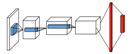
Model architecture:

1. conv1 + ReLU (32 filters of $8 \times 8$ with stride 4)
2. conv2 + ReLU (64 filters of $4 \times 4$ with stride 2)
3. conv3 + ReLU (64 filters of $3 \times 3$ with stride 1)
4. FC layer + ReLU(512)
5. FC layer with single output for each action

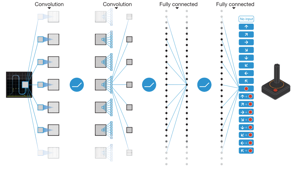
Training

• Optimizer: RMSProp
• $\epsilon$-greedy with $\epsilon$ annealed linearly from 1.0 to 0.1 over the 1st 1,000,000 frames, and fixed at 0.1 thereafter.
• Experience replay memory: 1,000,000 most recent frames.
• Training data: 50 million frames, i.e. ~38 days of game experiences
• Frame-skipping technique: select actions on every $k$-th frame instead of every frame, $k=4$.
• Tricks of Error clipping:
  Clip the error term from the update $r+\gamma \max_{a'} Q(s',a';\theta_i^{-}) - Q(s,a;\theta_i)$ to be in $[-1,1]$.

To perform experience replay, store the agents experience $e_t = (s_t, a_t, r_t, s_{t+1})$ at each time step $t$ in a dataset $D_t=\{e_1,\cdots,e_t\}$. During learning, at each time step, apply Q-learning updates on samples(or minibaches) of experience $(s,a,r,s')\sim \text{U(D)}$, drawn uniformly at random from the pool of stored samples. The target Q-network do periodical updates, so as to reduce the corerlations with the target. The loss function at iteration $i$:

$$L_{i}(\theta_i) = \mathbb{E}_{(s,a,r,s')\sim \text{U(D)}} \left[ \left( \underbrace{r + \gamma \max_{a'} Q(s',a';\theta_i^{-})}_\text{target Q-network} - Q(s,a;\theta_i) \right) \right]$$

where the target Q-network parameters $\theta_i^{-}$ are only updated with the Q-network parameters $\theta_i$ every $C$ steps, and are held fixed between individual updates.

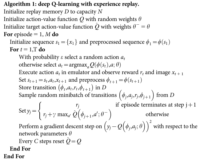
Deep Recurrent Q-Network(AAAI 2015)

Model architecture

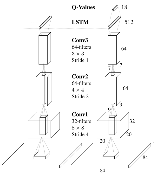
Replace the 1st FC layer with LSTMs^[3].
Model architecture:

1. conv1 + ReLU (32 filters of $8 \times 8$ with stride 4)
2. conv2 + ReLU (64 filters of $4 \times 4$ with stride 2)
3. conv3 + ReLU (64 filters of $3 \times 3$ with stride 1)
4. LSTM layer
5. FC layer with single output for each action

• No explicit improvement in comparison with Nature DQN
• Recurrency confers benefits with partial observability, when adapting at evaluation time if the quality of observation changes.
• Replacing LSTMs with 1st FC layer in DQN achive the best performance, intuitionally indicating that this allows LSTM direct access to the convolutional features.

Training

• Bootstrapped squential updates: randomly select episodes from the replay memory and updates begin at the beginning of the episode.
• Boostrapped random updates: randomly select eposides from the replay memory and updates begin at randomly points in the episode and proceed.

Both are viable and yield convergent policies with similar performance. Therefore, apply randomized update strategy.

Double DQN (AAAI 2016)

Problems:

• Q-learning algorithms lead to overestimation, since the $\max$ op employs the same values to both select and evaluate an action.

In DQN, the target Q-function is:

$$y_t^{DQN} = R_{t+1} + \gamma Q(S_{t+1}, \arg\max_a Q(S_{t+1},a;\pmb{\theta}_t); \pmb{\theta}_t)$$

In Double DQN, the target is:

$$y_t^{DDQN} = R_{t+1} + \gamma Q(S_{t+1}, \arg\max_a Q(S_{t+1},a;\pmb{\theta}_t); \pmb{\theta}_t^{-})$$

The weights of target Q-network $\pmb{\theta}_t^{-}$ stayed unchanged from DQN, and remains a periodic copy of the online network.

Prioritized Experience Replay

Background

• Online RL incrementally update the parameters while observing a stream of experience. This leads to problems:
  • strongly correlated updates break the i.i.d assumption of SGD algorithms;
  • rapid forgetting of possibly rare experiences.
• Experience replay uses a large sliding window replay memory, uniformly sampling experience transition from a replay memory at random. Experience replay frees online learning agents from processing transitions in the exact order that they are experienced, but suffer from sampling transitions with the same frequency that they are experienced.

Prioritized Experience Replay

• Intuition: RL agent can learn more effectively from some transitions than from others. Prioritized replay liberatres agents from considering transitions with the same frequency that they are experienced.

greedy TD-error prioritization

• Prioritize the experience transitions according to the magnitude of temporal-difference(TD) error $\delta$ ^[7], indicating how surprising or unexpected the transition is:

  $$\delta = | R_{t+1} + \gamma_{t+1} \max_{a'} q_{\theta}^{-}(S_{t+1,a'}) - q_\theta (S_t, A_t) |$$

• Implementation: priority queue with binary heap data structure.

  • the complexity of searching for the maximum $O(1)$
  • Update complexity $O(\log N)$

Stochastic prioritization

• The problems of greedy TD-error prioritization:

  1. TD errors are only updated for replayed transitions, resulting in that transitions with low TD error on first visit may not be replayed for a long time.
  2. It is sensitive to noise spikes(e.g. when rewards are stochastic), which can be exacerbated by bootstrapping where approximation errors appear as another source of noise.
  3. It focuses on a small subset of the experience: error shrink slowly, especially when using function approximation. This means initially high error transitions get replayed frequently, which is lack of diversity, making it prone to overfitting.

• Stochastic prioritization interpolates between pure greedy prioritization and uniform random sampling. We ensure the sampling probability is monotonic and guarantee non-zero prob. even for lowest-priority transition.

• Define the probability of sample transition $i$ as: $$P(i) = \frac{p_i^\alpha}{\sum_k p_k^\alpha}$$ where $p_i > 0$ is the priority of transition $i$. $\alpha$ determins how much prioritization is used, $\alpha = 0$ denotes to the uniform case.

Proportional prioritization

$$p_i = |\delta_i| + \epsilon$$

where $\epsilon$ is a small positive constant that prevents the edge-case of transitions not being revisited once their error is zero.

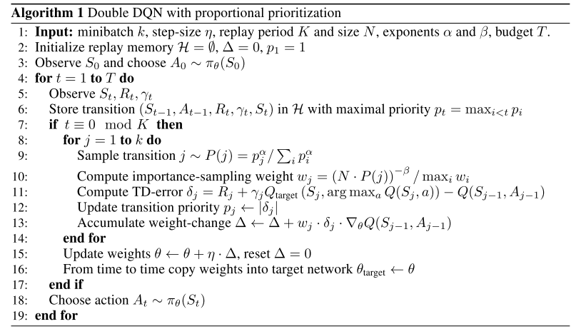
• Implementation: ‘sum-tree’ data structure.

Rank-based prioritization

$$p_i = \frac{1}{\text{rank}(i)}$$

where $\text{rank}(i)$ denotes the rank of transition $i$ according to $|\delta_i|$

Dueling DQN (ICML 2016)

Background

$Q$ measures the value of choosing a particular action when in this state:

$$Q^{\pi}(s,a) = \mathbb{E}[R_t \vert s_t=s, a_t=a, \pi]$$

$V$ measures how good it is to be in a particular state $s$:

$$V^{\pi}(s) = \mathbb{E}_{a \sim \pi(s)}[Q^\pi (s,a)]$$

The Advantage function $A^\pi$ measures the relative measure of the importance of each action:

$$A^\pi(s,a) = Q^{\pi}(s,a) - V^{\pi}(s)$$

Intuition:

• It is unnecessary to estimate the value of each action choice. In some states, it is of paramount importance to know which action to take, but in many other states the coice of action has no repercussion on what happens.
• In bootstrapping-based methods, the estimation of state values if of great importance for every state.

Model architecture

Dueling DQN decouples the value and advantage functions in separate streams ^[5].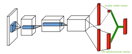

• Replace the 1st FC layer with two sequences(streams) of FC layers, which separately estimate the scalar state value $V(s;\theta, \beta)$ and $|\mathcal{A}|$-dimensional vector advantange $A(s,a;\theta,\alpha)$, where $\theta$ denotes parameters of conv layers, $\alpha$ and $\beta$ are the parameters of two streams of FC layers. Afterwards, combine both of them: $$Q(s,a; \theta,\alpha,\beta) = V(s;\theta,\beta) + A(s,a;\theta,\alpha)$$ To form the matrix form of $Q$, we need to replicate the scalar $V(s;\theta,\beta)$ $|\mathcal{A}|$ times, i.e. broadcasting the scalar value $V$ to $|\mathcal{A}|$ dimensions.

The above equation lead to identifiability that given $Q$ we cannot recover $V$ and $A$ uniquely. In other words, the resulting value remains the same if adding a constant substracted from $V$, to the advantage $\mathcal{A}$.
Thus, they forced the advantage function to zero by substracting the $\max$ value of $\mathcal{A}$:

$$Q(s,a; \theta,\alpha,\beta) = V(s;\theta,\beta) + \left( A(s,a;\theta,\alpha) - \max_{a' \in |\mathcal{A}|} A(s,a'; \theta, \alpha) \right)$$

Here, for $a^* = \arg\max_{a' \in \mathcal{A}} Q(s,a';\theta,\alpha,\beta) = \arg\max_{a' \in \mathcal{A}} A(s,a';\theta,\alpha)$.

An alternative way is replace $\max$ with average op:

$$Q(s,a; \theta,\alpha,\beta) = \underbrace{V(s;\theta,\beta)}_\text{scalar} + \left( \underbrace{A(s,a;\theta,\alpha)}_{|\mathcal{A}|-\text{dimensional vector}} - \underbrace{\frac{1}{|\mathcal{A}|} \sum_{a'} A(s,a'; \theta, \alpha)}_\text{scalar} \right)$$

This alternative loses the original semantics of $V$ and $A$ since they are off-target by a constant, but it increases the stabiliity of the optimization.

The $\text{softmax}$ version’s performance matched the above average version.

Rainbow DQN (AAAI 2018)

• RainBow DQN integrates the ingredients of Double DQN, Prioritized replay, Dueling DQN, multi-step learning, distributional RL and Noisy Net^[6].

• Apply Adam optimizer: less sensitive to the choice of learning rate then RMSProp.

• The ablation studies illustrate that prioritized replay and multi-step learning were the two most crucial components of Rainbow, in that removing either component caused a large drop.

• Other ingredients to research: Bootstrapped DQN, instrinsic motivation, count-bsed exploration.

References

---

1. 1.Mnih, V., Kavukcuoglu, K., Silver, D., Rusu, A. A., Veness, J., Bellemare, M. G., ... & Petersen, S. (2015). Human-level control through deep reinforcement learning. Nature, 518(7540), 529. ↩
2. 2.Mnih, V., Kavukcuoglu, K., Silver, D., Graves, A., Antonoglou, I., Wierstra, D., & Riedmiller, M. (2013). Playing atari with deep reinforcement learning). arXiv preprint arXiv:1312.5602. ↩
3. 3.Hausknecht, M., & Stone, P. (2015, September). Deep recurrent q-learning for partially observable mdps. In 2015 AAAI Fall Symposium Series. ↩
4. 4.Van Hasselt, H., Guez, A., & Silver, D. (2016, March). Deep reinforcement learning with double q-learning. In Thirtieth AAAI Conference on Artificial Intelligence. ↩
5. 5.Wang, Z., Schaul, T., Hessel, M., Hasselt, H.V., Lanctot, M., & Freitas, N.D. (2016). Dueling network architectures for deep reinforcement learning. ICML. ↩
6. 6.Hessel, M., Modayil, J., Van Hasselt, H., Schaul, T., Ostrovski, G., Dabney, W., ... & Silver, D. (2018, April). Rainbow: Combining improvements in deep reinforcement learning. In Thirty-Second AAAI Conference on Artificial Intelligence. ↩
7. 7.Schaul, T., Quan, J., Antonoglou, I., & Silver, D. (2015). Prioritized experience replay. arXiv preprint arXiv:1511.05952. ↩