Normalization in Neural Networks: A Summary !

A survey of the normalization tricks in Neural Networks.

Feature Normalization

Data Preprocessing

• Normalization: subtract the mean of the input data from every feature, and scale by its std deviation.

  $$\hat{x}_i^n = \frac{x_i^n - \text{mean}(x_i)}{\text{std}(x_i)}$$

• PCA (Principal Components Analysis)

  • Decorrelate the data by projecting onto the principal components
  • Also possible to reduce dimensionality by only projecting onto the top $P$ principal components.

• Whitening

  • Decorrelate by PCA
  • Scale each dimension

Batch Normalization

Problems:

• Internal covariate shift: the distribution of each layer’s inputs changes during training, as the parameters of the previous layers change. This slows down the training by requiring lower learning rates and careful parameter initialization， and make it notoriously hard to train models with saturating nonlinearities.

• Intuition : To reduce the internal covariate shift, by fixing the distribution of the layer inputs $x$.
• Idea: The NN converges faster if the inputs is whitened, i.e. linearly transformed to have zero mean and unit variance, and decorrelated.

Solution: batch normalization (BN) ^[1].

• Use mini-batch statistics to normalize activations of each layer.
• Parameter $\gamma$ and $\beta$ can scale and shift (a.k.a. bias) the normalized activations.
• BatchNorm depends on the current training example - and on examples in mini-batch (for computing mean and variance)

• Training

  • Set parameters $\gamma$ and $\beta$ by gradient descent - require gradients $\frac{\partial E}{\partial \gamma}$ and $\frac{\partial E}{\partial \beta}$
  • TO backpropagate gradients through the batchNorm layer aliso require: $\frac{\partial E}{\partial \hat{u}}$, $\frac{\partial E}{\partial \sigma^2}$, $\frac{\partial E}{\partial \mu}$, $\frac{\partial E}{\partial u_i}$

• Runtime: use the sample mean and variance computed over the complete training data as the mean and variance parameters for each layer - fixed transform:

$$\hat{u}_i = \frac{u_i - \text{mean}(u_i)}{\sqrt{\text{Var}(u_i) + \epsilon}}$$

• Backprop: see ^[2]

• Input: values of $x$ over a mini-batch: $\beta = {x_{1 \cdots m}}$

• Outputs: ${y_i = BN_{\gamma, \beta} (x_i)}$

  mini-batch mean:

  $$\mu_{\beta} \leftarrow \sum_{i=1}^m x_i$$

  mini-batch variance:

  $$\sigma_{\beta}^2 \leftarrow \frac{1}{m} \sum_{i=1}^m (x_i - \mu_{\beta})^2$$

  normalize:

  $$\hat{x} \leftarrow \frac{x_i - \mu_{\beta}}{\sqrt{\sigma_{\beta}^2 + \epsilon}}$$

  scale and shift:

  $$y_i \leftarrow \gamma \hat{x_i} + \beta \equiv \text{BN}_{\gamma, \beta}(x_i)$$

• Parameters: $\gamma$ and $\beta$ are trainable parameters with size $C$ (where $C$ is the channel size). By default, the elements of $\gamma$ are set to 1s and the elements of $\beta$ are set to 0s.

class BatchNorm(nn.Module):
    # `num_features`: the number of outputs for a fully-connected layer
    # or the number of output channels for a convolutional layer. `num_dims`:
    # 2 for a fully-connected layer and 4 for a convolutional layer
    def __init__(self, num_features, num_dims):
        super().__init__()
        if num_dims == 2:
            shape = (1, num_features)
        else:
            shape = (1, num_features, 1, 1)
        # The scale parameter and the shift parameter (model parameters) are
        # initialized to 1 and 0, respectively
        self.gamma = nn.Parameter(torch.ones(shape))
        self.beta = nn.Parameter(torch.zeros(shape))
        # The variables that are not model parameters are initialized to 0 and 1
        self.moving_mean = torch.zeros(shape)
        self.moving_var = torch.ones(shape)

    def forward(self, X):
        # If `X` is not on the main memory, copy `moving_mean` and
        # `moving_var` to the device where `X` is located
        if self.moving_mean.device != X.device:
            self.moving_mean = self.moving_mean.to(X.device)
            self.moving_var = self.moving_var.to(X.device)
        # Save the updated `moving_mean` and `moving_var`
        Y, self.moving_mean, self.moving_var = batch_norm(
            X, self.gamma, self.beta, self.moving_mean, self.moving_var,
            eps=1e-5, momentum=0.9)
        return Y

• Benefits
  • Make training many-layered networks easier.
    • allow higher learning rates
    • weight initialization less cruc
  • Can act like a regularizer: can reduce need for techniques like dropout

Pros:

• Prevent small changes to the parameters from amplifying into larger and suboptimal changes in activations in gradients, e.g. it prevents the training from getting stuck in the saturated regimes of nonlinearities.
• More resilient to the the parameter scale. Large learning rates may increase the scale of layer parameters, which then amplify the gradient during back-propagation and lead to the model explosion.

Drawbacks:

• BN performs different in training and test time.
• It is not legitimate at inference time, so the mean and variance are pre-computed from the training set, often by running average.

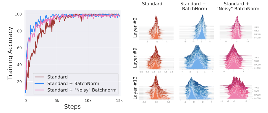
Different opinion at NIPS 2018: ^{<span class=”hint—top hint—error hint—medium hint—rounded hint—bounce” aria-label=”How Does Batch Normalization Help Optimization?}

“>[7]</span></a></sup>

• Argument: BatchNorm cannot handle internal covariate shift, i.e. no link between the performance gain of BatchNorm and the reduction of internal covariate shift. It makes the optimization landscape significantly smoother.
• Experiment: inject random noise with a severe covariate shift after batch normalization, which still performs better when training.

• BatchNorm makes the landscape significantly more smooth: improvement in the Lipschitzness of the loss function. i.e. the loss exhibits a significantly better “effective” $\beta$-smoothness.
  1. Reparametrization make it more stable (in the sense of loss Lipschitzness)
  2. more smooth (in the sense of “effective” $\beta$-smoothness of the loss)

Layer Normalization

Problems:

• Batch normalization is dependent on the mini-batch size, i.e. cannot apply on extremely small minibatches.
• Not obvious how to apply on RNNs. It can easily applied on FFNN because of the fixed length of inputs.

Solution: layer normalization (LN)^[3].

• Compute the layer normalization statistics over all hidden units in the same layer: $$\mu^l = \frac{1}{H} \sum_{i=1}^{H} \alpha_i^l$$

$$\sigma^l = \sqrt{\frac{1}{H} \sum_{i=1}^H (a_i^l - \mu^l)^2 }$$

where $H$ denotes the # of hidden units in a layer. Under layer norm, all hidden states in a layer share the same normalization terms $\mu$ and $\sigma$. Furthermore, it does not impose any constraint on the size of a mini-batch, and it can be used in the pure online regime with batch size 1.

$$y = \frac{x-\mathbb{E}[x]}{\sqrt{\textrm{Var}[x] + \epsilon}} * \gamma + \beta$$

where the mean and standard deviation are calculated seperately over the last certain number dimensions which have to be of the shape specified by the last dim. $\gamma$ and $\beta$ are learnable affine transform parameters. Denoting the hidden dim as $D$, the parameter count of LN is $2*D$.

import torch
import torch.nn as nn
import torch.nn.functional as F

class LayerNorm(nn.Module):
    """ layer norm"""

    def __init__(self, features, eps=1e-6):
        super(LayerNorm, self).__init__()
        self.weight = nn.Parameter(torch.ones(features))
        self.bias = nn.Parameter(torch.zeros(features))
        self.eps = eps

    def forward(self, x):
        mean = x.mean(-1, keepdim=True)
        std = x.std(-1, keepdim=True)
        return self.weight * (x - mean) / (std + self.eps) + self.bias
        

Layer Normalization on RNNs

In a std RNN, $h^{t-1}$ denotes previous hidden states, $x^t$ represents the current input vector:

$$\pmb{a}^t = W_{hh}\pmb{h}^{t-1} + W_{xh}\pmb{x}^t$$

Do layer normalization:

$$\pmb{h}^t = f(\frac{\pmb{g}}{\sigma^t} \odot(\pmb{a}^t - \mu^t) + \pmb{b})$$ $$\mu^t = \frac{1}{H} \sum_{i=1}^H a_i^t$$ $$\sigma^t = \sqrt{\frac{1}{H} \sum_{i=1}^H (a_i^t - \mu^t)^2}$$

where $W_{hh}$ is the recurrent hidden to hidden weights and $W_{xh}$ are the bottom up input to hidden weights, $\odot$ is element-wise multiplication between to vectors.

Differences between batch normalization and layer normalization:

• LN: neurons in the same layer have the same mean and variance; different input samples have different mean and variance.
• BN: input samples in the same batch have the same mean and variance; different neurons.

Unlike BN, layer norm performs exactly the same computation at training and test times.

RMSNorm

Root Mean Square Normalization (RMSNorm)^[8] hypothesize that the rescaling invariance is the reason for success of LayerNorm, rather than re-centering invariance. RMSNorm rescales invariance and regularizes the summed inputs using root mean square (RMS) statistic:

$$\begin{equation} \bar{a}_i=\frac{a_i}{\mathrm{RMS}(\mathbf{a})}g_i,\quad\text{where RMS}(\mathbf{a})=\sqrt{\frac1n\sum_{i=1}^na_i^2}. \end{equation}$$

RMSNorm simplifies LayerNorm by totally removing the mean statistic at the cost of sacrificing the invariance that mean normalization affords. When the mean of summed inputs is zero, RMSNorm is exactly equal to LayerNorm.

Implementation:

# Code source: https://github.com/bzhangGo/rmsnorm/blob/master/rmsnorm_torch.py
import torch
import torch.nn as nn


class RMSNorm(nn.Module):
    def __init__(self, d, p=-1., eps=1e-8, bias=False):
        """
            Root Mean Square Layer Normalization
        :param d: model size
        :param p: partial RMSNorm, valid value [0, 1], default -1.0 (disabled)
        :param eps:  epsilon value, default 1e-8
        :param bias: whether use bias term for RMSNorm, disabled by
            default because RMSNorm doesn't enforce re-centering invariance.
        """
        super(RMSNorm, self).__init__()

        self.eps = eps
        self.d = d
        self.p = p
        self.bias = bias

        self.scale = nn.Parameter(torch.ones(d))
        self.register_parameter("scale", self.scale)

        if self.bias:
            self.offset = nn.Parameter(torch.zeros(d))
            self.register_parameter("offset", self.offset)

    def forward(self, x):
        if self.p < 0. or self.p > 1.:
            norm_x = x.norm(2, dim=-1, keepdim=True)
            d_x = self.d
        else:
            partial_size = int(self.d * self.p)
            partial_x, _ = torch.split(x, [partial_size, self.d - partial_size], dim=-1)

            norm_x = partial_x.norm(2, dim=-1, keepdim=True)
            d_x = partial_size

        rms_x = norm_x * d_x ** (-1. / 2)
        x_normed = x / (rms_x + self.eps)

        if self.bias:
            return self.scale * x_normed + self.offset

        return self.scale * x_normed

Instance Normalization

Image style transfer

• Transfer a style from one image to another, which relies more on a specific instance rather than a batch.

Solution:

• Instance normalization (IN) ^[4] , a.k.a. contrast normalization, do instance-specific normalization rather than batch normalization.
• It performs the same at training and test time.

$$y_{tijk} = \frac{x_{tijk} - \mu_{ti}}{\sqrt{\sigma^2_{ti}+ \epsilon}}$$ $$\mu_{ti} = \frac{1}{HW} \sum_{l=1}^W \sum_{m=1}^H x_{tilm}$$ $$\sigma^2_{ti} = \frac{1}{HW} \sum_{l=1}^W \sum_{m=1}^H (x_{tilm} - mu_{ti})^2$$

Group Normalization

Problems:

• BN’s error increases rapidly when the batch size becomes smaller because of inaccurate batch statistics estimation.

Solution: Group Normalization (GN)^[5]. GN divides the channels into groups and computes within each group the mean and variance for normalization. GN’s computation is independent of batch sizes, and its accuracy is stable in a wide range of batch sizes.

GN divides the set $S_i$ as:

$$S_i = \{k \vert k_N = i_N, \lfloor \frac{k_C}{C/G} \rfloor = \lfloor \frac{i_C}{c/G} \rfloor \}$$

where $G$ is the number of groups, $C/G$ is the number of channels per group, $k$, $i$ is the index. GN compute the $\mu$ and $\sigma$ along the (H,W) axes and along a group by $\frac{C}{G}$ channels.

def GroupNorm(x, gamma, beta, G, eps=1e-5):
	"""
    : param x: input features with shape [N,C,H,W]
    : param gamma, beta: scale and offset, with shape [1,C,1,1]
    : param G: number of groups for GN
    """
	
    N,C,H,W = x.shape
    x = tf.reshape(x, [N, G, C//G, H, W]
    
    mean, var = tf.nn.moments(x, [2,3,4], keep_dims=True)
    x = (x - mean) / tf.sqrt(var + eps)
    
    x = tf.reshape(x, [N, C, H, W])
    return x* gamma + beta

Switchable Normalization

Problems:

• Existing BN, IN, LN employed the same normalizer in all normalization layers of an entire network, rendering suboptimal performance.
• Different normalizers are used to solve different tasks, making model design cumbersome.

Solution:

• Switchable Normalization (SN) ^[6]. It combines three distinct scopes to compute statistics (i.e. mean and variance): channel-wise, layer-wise and minibatch-wise, by using IN, LN and BN respectively. SN switches them by learning their importance weights end-to-end.

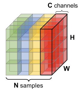
Given a 4D tensor [N,C,H,W], denoting the # of samples, # of channels, heights and weights. Let $h_{ncij}$ and $\hat{h_{ncij}}$ be a pixel before and after the normalization, where $n \in [1,N]$, $c \in [1,C]$, $i \in [1,H]$ and $j \in [1,W]$. $\gamma$ and $\beta$ are a scale and shift parameter respectively, $\epsilon$ is a small constant to preserve numerical stability.

$$\hat{h_{ncij}} = \gamma \frac{h_{ncij} - \sum_{k \in \omega}w_k\mu_k}{ \sqrt{ \sum_{k \in \omega} w'_k \sigma_k^2 + \epsilon}} + \beta$$

where $\Omega = { \text{in, ln, bn} }$:

$$\mu_{in} = \frac{1}{HW} \sum_{i,j}^{H,W} h_{ncij}, \quad \sigma_{in}^2 = \frac{1}{HW} \sum_{i,j}^{H,W} (h_{ncij} - \mu_{in})^2$$ $$\mu_{ln} = \frac{1}{C} \sum_{c=1}^{C} \mu_{in}, \quad \sigma_{ln}^2 = \frac{1}{C} \sum_{c=1}^{C} (\sigma_{in}^2 + \mu_{in}^2)^2 -\mu_{ln}^2$$ $$\mu_{bn} = \frac{1}{N} \sum_{n=1}^{N} \mu_{in}, \quad \sigma_{bn}^2 = \frac{1}{N} \sum_{n=1}^{N} (\sigma_{in} + \mu_{in})^2 -\mu_{bn}^2$$

Different normalizers estimate statistics along different axes.

def SwitchableNorm(x, gamma, beta, w_mean, w_var, eps=1e-5):
	"""
    x: shape [N,C,H,W]
    """
    # Instance Norm
    mean_in = np.mean(x, axis=(2,3), keepdims=True)
    var_in = np.var(x, axis=(2,3), keepdims=True)
    
    # Layer Norm
    mean_ln = np.mean(x, axis=(1,2,3), keepdims=True)
    var_ln = np.var(x, axis=(1,2,3), keepdims=True)
	
    # Batch Norm
    mean_bn = np.mean(x, axis=(0,2,3), keepdims=True)
    var_bn = np.var(x, axis=(0,2,3), keepdims=True)
	
    # Switchable Norm
    mean = w_mean[0]*mean_in + w_mean[1]*mean_ln + w_mean[2]*mean_bn
    var = w_var[0]*var_in + w_var[1]*var_ln + w_var[2]*var_bn
    
    x_normalized = (x-mean) / np.sqrt(var + eps)
    return gamma * x_normalized + beta

Comparison

The mini-batch data has the shape [N, C, H, W], where

• $N$ is the batch axis
• $C$ is the channel axis (rgb for image data)
• $H$ and $W$ are the spatial hight and weight axis

Comparison:

• Batch Norm is applied on batch, normalizing along (N, H, W) axis, i.e. compute the mean and variance for the whole batch of input data. (It performs badly for small batch size)
• Layer Norm is on channel, normalizing along (C,H,W) axis, i.e. it is independent with batch dimension, by normalizing the neurons. (It is obvious for RNNs).
• Instance Norm is applied on image pixel, doing normalization along (H,W) axis, i.e. compute $\mu$ and $\sigma$ for each sample and channel. (It is for style transfer)
• Group Norm: divide the channel into groups, normalizing along the (H,W) axis and along a group of $\frac{C}{G}$ channels.
• Switchable Norm: dynamically learn weights for IN/LN/BN statistics in the e2e manner (c.f. ELMo).

References

---

1. 1.Batch Normalization: Accelerating Deep Network Training by Reducing Internal Covariate Shift ↩
2. 2.What does the gradient flowing through batch normalization looks like ? ↩
3. 3.Layer normalization ↩
4. 4.Instance Normalization: The Missing Ingredient for Fast Stylization ↩
5. 5.Group Normalization ↩
6. 6.Differentiable learning-to-normalize via Switchable Normalization ↩
7. 7.How Does Batch Normalization Help Optimization? ↩
8. 8.Zhang, Biao, and Rico Sennrich. "Root mean square layer normalization." Advances in Neural Information Processing Systems 32 (2019). ↩