Notes of lectures by D. Silver.A brief introduction of MDPs.
Markov Decision Processes
Intro to MDPs
MDP formally describe an environment for RL, where the environment is fully observable. i.e. the current state completely characterizes the process.
Almost all RL problems can be formalized as MDPs, e.g.
- Optimal control primarily deals with continuous MDPs
- Partially observable problems can be converted into MDPs
- Bandits are MDPs with one state
Markov Process
Markov property
“The future is independent of the past given the present”
Definition: a state is Markov iff
- The state captures all relevant information from the history.
- Once the state is known, the history maybe thrown away, i.e. the state is sufficient statistic of the future.
State Transition Matrix
For a Markov state $s$ and successor state $s’$, the state transition probability is :
Sate transition matrix $\mathcal{P}$ defines transition probabilities from all sates $s$ to all successor states $s’$
where each row of the matrix sums to 1.
Markov Process
A Markov process is a memoryless random process, i.e. a sequence of random state $S_1$, $S_2$, … with the Markov property.
Definition: a Markov Process (or Markov Chain) is a tuple $<\mathcal{S}, \mathcal{P}>$, where $\mathcal{S}$ is a (finite) set of states, $\mathcal{P}$ is a state transition probability matrix,
Markov Reward Process
A Markov reward process is a Markov chain with values.
Definition: A MRP is a tuple $\mathcal{S}, \mathcal{P}, \mathcal{R}, \mathcal{\gamma}$
- $\mathcal{S}$ is a finite set of states
- $\mathcal{P}$ is a state transition probability matrix,
- $\mathcal{R}$ is a reward function,
- $\mathcal{\gamma}$ is a discount factor,
Return
The return is the total discounted reward from time-step $t$.
- The discount $\gamma \in [0,1]$ is the present value of future rewards.
- The value of receiving reward $R$ after $k+1$ time stems is $\gamma^k R$.
- This values immediate reward above delayed reward
- $\gamma$ close to 0 leads to “myopic” evaluation
- $\gamma$ close to 1 leads to “far-sighted” evaluation
Why discount ?
Most MRP, MDP are discounted. Why?
- Mathematically convenient to discount rewards.
- Avoids infinite returns in cyclic Markov processes.
- Uncertainty about the future may not be fully represented.
- If the reward is financial, immediate rewards may earn more interest than delayed rewards
- Animal/human behavior shows preference for immediate reward
- It is sometimes possible to use undiscounted MRP (i.e. $\gamma = 1$), e.g. if all sequences terminate.
Value Function
The value function $v(s)$ gives the long-term value of state $s$
Definition: the state value function $v(s)$ of an MRP is the expected return starting from state $s$:
Bellman Equation for MRPs
The value function can be decomposed into two parts:
- immediate reward
- discounted value of successor state

Bellman equation in matrix form
where $v$ is a column vector with one entry per state
Solving the Bellman equation
The Bellman equation is a linear equation
Computational complexity $\rightarrow O(n^3)$ for $n$ states
- Direct solution is only possible for small MRPs
- For large MRPs, iterative methods:
- Dynamic programming
- Monte-Carlo evaluation
- Temporal-Difference learning
Markov Decision Process
Markov Decision Process(MDP): a Markov reward process with decisions.
An MDP is a tuple $<\mathcal{S}, \mathcal{A}, \mathcal{P}, \mathcal{R}, \mathcal{\gamma}>$
- $\mathcal{S}$ is a finite set of states
- $\mathcal{A}$ is a finite set of actions
- $\mathcal{P}$ is a state transition probability matrix
- $\mathcal{R}$ is a reward function,
- $\gamma$ is a discount factor $\gamma \in [0,1]$
Policies
A policy $\pi$ is a distribution over actions given states
- A policy fully defines the behavior of an agent.
- MDP policies depends on the current state (not the history), i.e. Policies are stationary (time-independent)
Given an MDP $\mathcal{M} = <\mathcal{S}, \mathcal{A}, \mathcal{P}, \mathcal{R}, \mathcal{\gamma}>$ and a policy $\pi$
- The state sequence $S_1, S_2,…$ is a Markov process $<\mathcal{S}, \mathcal{P}^{\pi}>$
- The state and reward sequence is a markov reward process $<\mathcal{S}, \mathcal{P}^{\pi}, \mathcal{R}^{\pi}, \gamma>$
where
Value Function
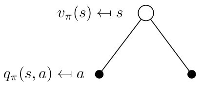
The state-value function of an MDP is the expected return starting from state $s$, and then following policy $\pi$
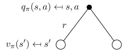
The action-value function is the expected return starting from state $s$, taking action $a$, and then following policy $\pi$
Bellman Expectation Equation
The state-value function can again be decomposed into immediate reward plus discounted value of successor state:
The action-value function can similarly be decomposed:
Bellman Expectation equation for $V^{\pi}$
(Eq. 1)

(Eq. 2)

Bellman Expectation equation for $Q^{\pi}$
(Eq. 1)

(Eq. 2)

Matrix form
The Bellman expectation equation can be expressed concisely using the induced MRP:
with direct solution
Optimal Value Function
The optimal state-value function is the maximum value function over all policies:
The optimal action-value function is the maximum action-value function over all policies
An MDP is solved when we know the optimal value fn.
Optimal Policy
Define a partial ordering over policies
Finding an optimal policy, by maximizing over
Solving the Bellman Optimality Equation
- Bellman Optimal Equation is non-linear
- No closed form solution (in general)
- Many iterative solution methods
- Value iteration
- Policy iteration
- Q-learning
- Sarsa
Extensions to MDPs
Infinite MDPs
- Countably infinite state and/or action spaces: straightforward
- Continuous state and/or action spaces
- Closed form for linear quadratic model (LQR)
- Continuous time
- Requires partial differential equations
- Hamilton-Jacobi-Bellman (HJB) equation
- LImiting case of bellman equation as time-step $\rightarrow 0$
POMDPs
A POMPD is an MDP with hidden states. It is a hidden Markov model with actions.
A POMDP is a tuple $<\mathcal{S}, \mathcal{A},\mathcal{O},\mathcal{P},\mathcal{R},\mathcal{Z},\mathcal{\gamma}>$
- $\mathcal{S}$ is a finite set of states
- $\mathcal{A}$ is a finite set of actions
- $\mathcal{O}$ is a finite set of observations
- $\mathcal{P}$ is a state transition probability matrix
- \mathcal{R} is a reward function,
- $\mathcal{Z}$ is an observation function
- $\gamma$ is a discount factor $\gamma \in [0,1]$
