A brief introduction of the probability theory and the information theory.
Introduction
Bayesian interpretation models the uncertainty about the events.
Probability theory
Discrete random variables
We denote the probability of the event that $X=x$ by $p(X=x)$, ro just $p(x)$ for short. The expression $p(A)$ denotes the probability that the event $A$ is true. Here $p()$ is called a probability mass function (pmf).
Fundamental rules
Union of two event:
Joint probabilities:
Marginal distribution:
Chain rule of probability:
Conditional probability:
Bayes rule (a.k.a Bayes Theorem):
Continuous random variables
Cumulative distribution function (cdf) of $X$: define .
probability density function (pdf): define
Mean and Variance
Mean (expected value)
Let $\mu$ denote the mean(expected value).
- For discrete rv’s:
- For continuous rv’s:
Variance
Let denote the measure of the “spread of a distribution”.
Derive a useful result:
The standard deviation is:
Common discrete distributions
The binomial and Bernoulli distributions
Suppose we toss a coin $n$ times. Let $X \in { 0,…,n }$ be the number of heads. If the probability of heads is $\theta$, then X has a binomial distribution: $\text{X} ~ \text{Bin}(n, \theta)$
where
is the number of ways to choose $k$ items from $n$ (a.k.a. binomial coefficient, pronounced “n choose k”).
Suppose we only toss a coin only once. Let be a binary random variable, with the probability of “success” or “heads” of $\theta$. We say that $X$ has a Bernoulli distribution: , where the pmf is defined as:
The multinomial and multinoulli distributions
The binomial distribution only model the outcomes of coin tosses (2 results per round). We use multinomial distribution to model the outcomes of tossing a $K$-sided die. Let $\mathbf{x} = (x_1,…,x_K)$ be a random vector, where $x_j$ is the number of times side $j$ of the die occurs. The pmd is:
where is the probability that side $j$ shows up, and the multinomial coefficient () is:
Suppose $n = 1$, we rolling a $K$-sided dice once. This is called one-hot encoding .
The Poisson distribution
With parameter $\lambda > 0$, $X \sim \text{Poi}(\lambda)$, if its pmf is:
where the first term is just the normalization constant.
The empirical distribution
Given a set of data , define the empirical distribution (a.k.a. empirical measure):
where is the Dirac measure, defined by:
Common continuous distributions
Gaussian (normal) distribution
Let $X \sim \mathcal{N}(\mu, \sigma^2)$ denote
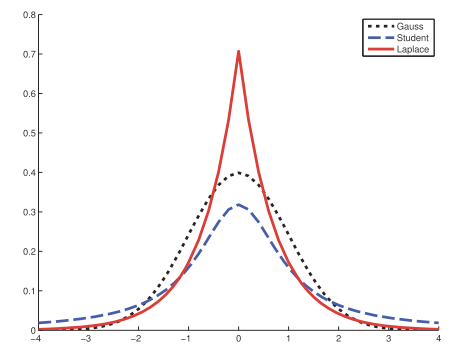
The precision of a Gaussian, i.e. the inverse variance . A high precision means a narrow distribution (low variance) centered on $\mu$.
- Problems: Gaussian distribution is sensitive to outliers, since the log-probability only decays quadratically with the distance from the center.
More robust: Student $t$ distribution.
Laplace distribution
A.k.a. double-sided exponential distribution.
Here $\mu$ is a location parameter and $b>0$ is a scale parameter.

Gamma distribution
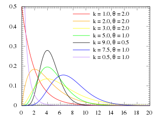
The gamma distribution is a flexible distribution for positive real valued rv’s, $x>0$.
where $\gamma(a)$ is the gamma function:

Beta distribution
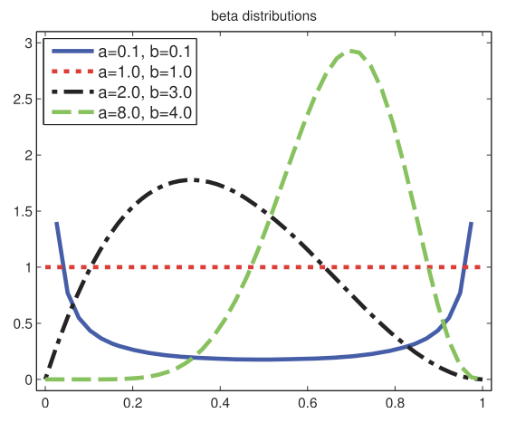
The beta distribution has support over the interval [0,1]:
Here $B(p,q)$ is the beta function,

Pareto distribution
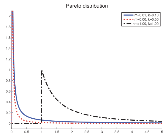
The Pareto distribution is used to model the distribution of quantities that exhibit long tails (heavy tails).
For example, the most frequent ward in English occurs approximately twice as often as the second most frequent word, which occurs twice as oten as the fourth most frequent word. This is Zipf’s law.
Its pdf:

Joint probability distributions
A joint probability distribution has the form for a set of $D > 1$ variables, and models the (stochastic) relationships between the variables.
Covariance and correlation
Covariance between two rv’s X and Y measures the degree to which X and Y are (linearly) related.
If $\mathbf{x}$ is a $d$-dimensional random vector, its covariance matrix is defined to be symmetric, positive definite matrix:
Covariance $\in [0, \infty]$. Pearson correlation coefficient use normalized measure with a finite upper bound:
Acorrelation matrix has the form:
where $\text{corr}[X,Y] \in [-1, 1]$.
independent $\Rightarrow$ uncorrelated,
uncorrelated $\nRightarrow$ independent.
Measure the dependence between rv’s: mutual information.
Multivariate Gaussian
The Multivariate Gaussian or multivariate normal (MVN) is the most widely used pdf for continuous variables.
Its pdf:
where $\mathbf{\mu} = \mathbb{E}[\mathbf{x}] \in \mathbb{R}^D$ is the mean vector, and $\Sigma = \text{cov}[\mathbf{x}]$ is the $D /times D$ covariance matrix. The precision matrix or concentration matrix is the inverse covariance matrix, . The normalization constant $(2\pi)^{-D/2} |\mathbf{\Lambda}^{1/2}|$ just ensure that the pdf integrates to 1.
Multivariate Student $t$ distribution
Dirichlet distribution
Transformations of random varianbles
Linear transformation
Suppose $f()$ is a linear function:
Linearity of expectation:
where $\mathbf{\mu}=\mathbb{E}[\mathbf{x}]$.
Covariance:
where $\Sigma = \text{cov}[\mathbf{x}]$
If $f()$ is a scalar-valued function, $f(\mathbf{x}) = \mathbf{a}^T \mathbf{x} + b$, the mean is:
The covariance:
Central limit theorem
Consider $N$ random variables with pdf’s $p(xi)$, each with mean $\mu$ and variance $\sigma^2$. We assume each variable is iid(independent and identically distributed). Let $$S_N = \sum{i=1}^N X_i$$ be the sum of the rv’s.
As $N$ increases, the distribution of this sum approaches
Hence the distribution of the quantity
converges to the standard normal, where is the sample mean. (central limit theorem)
Monte Carlo approximation
Computing the distribution of a function of an rv using the change of variables formula is difficult.
Monte Carlo approximation: First generate $S$ samples from the distribution, called them . Given the samples, we approximate the distribution of $f(X)$ by using the empirical distribution of .
Approximate the expected value with the arithmetic mean of the function applied to the samples:
where . This is called Monte Carlo integration.
Information theory
Information theory represents data in a compact fashion, as well as with transmitting and storing it in a way that is robust to errors.
Entropy
Entropy of a rv $X$ with distribution $p$, denoted by $\mathbb{H}(X)$, is a measure of its uncertainty. For a discrete rv with $K$ states:
Usually we use log base 2, where it is called bits (short for binary digits); whereas log base $e$ is called nats. The discrete distribution with maimum entropy is the uniform distribution.
KL divergence
Kullback-Leibler (KL) divergence or relative entropy: measures the dissimilarity of two probability distributions, $p$ and $q$.
where the sum gets replaced by an integral for pdf’s.
where $\mathbb{H}(p,q)$ is called the cross entropy.
Cross entropy: the average number of bits needed to encoder data coming from a source with distribution $p$ when we use model $q$ to define our codebook, i.e. KL divergence is the avarage number of extra bits needed to encode the data, due to the fact that we use distribution $q$ to encoder the data instead of the true distribution $p$.
The “extra number of bits” interpretation implies that $\mathbb{KL}(p||q) \geq 0 $, and KL is only equal to zero iff $q = p$.
Information inequality:
Mutual information
Mutual Information (MI): determine how similar the joint distribution $p(X,Y)$ is to the factored distribution $p(X)p(Y)$.
where $\mathbb{I}(X;Y) \geq 0$ woth equality iff $p(X,Y) = p(X) p(Y)$, i.e. the MI is zero iff the variables are independent.
where is the conditional entropy, defined as .
Hence we interpret the MI between $X$ and $Y$ as the reduction in uncertainty about $X$ after observing $Y$, or by symmetry, the reduction in uncertainty about $Y$ after observing $X$.
Pointwise mutual information (PMI): measures the discrepancy between events $x$ and $y$ occurring together compared to what would be expected by chance.
The MI of $X$ and $Y$ is the expected value of the PMI.
We can interpret that PMI is the amount we update the prior $p(x)$ into the posterior $p(x|y)$, or equivalently update the prior $p(y)$ into $p(y|x)$.
