Attention mechanism has been widely applied in natural langugage processing and computer vision tasks.

Attention mechanism

Background: what is WRONG with seq2seq?

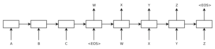
Encoder-decoder architecture:
Encode a source sentence into a fixed-length vector from which a decoder generates a translation.^[3]

Seq2seq models encode an input sentence of variable length $(x_1,...,x_T)$ into a fixed-length vector representation $c$ (a.k.a sentence embedding, “thought” vector), by apply one LSTM to read the input sentence, one timestep at a time. The representation vector $c$ is expected to well capture the meaning of the source sentence.
Then decode the vector representation $v$ to the target sentence $(y_1,...,y_{T'})$ with another LSTM whose initial hidden state is the last hidden state of the encoder (i.e. the representation of the input sentence: $c$). ^[1]

$p(y_1,...,y_{T'} | x_1,...,x_T) = \prod_{t=1}^{T'} p(y_t|c,{y_1,...,y_{t-1}})$ $p(y_t|c,{y_1,...,y_{t-1}}) = g(y_{t-1}, s_t, c)$

where $g$ is a RNN that outputs the probability of $y_t$ , and $s_t$ is the hidden state of the RNN. $c$ is the fixed-length context vector for the input sentence.

Drawbacks: The fixed-length context vector $c$ is incapable of remembering long sentences^[2]. It will forget the former part when processing the latter sequence. Sutskever et al.(2014)^[1] proposed a trick that only reversing the order of source sentences rather than target sentences could be of benefit for MT.

Basic encoder-decoder architecture compresses all the necessary information of a source sentence into a fixed-length vector. This may be incapable of coping with long sentences, especially those that are longer than the sentences in the training corpus ^[3]. The performance of basic encoder-decoder drops rapidly as the length of an input sentence increases ^[4].

Thus attention mechanism is proposed to tackle this problem.

Attention mechanism

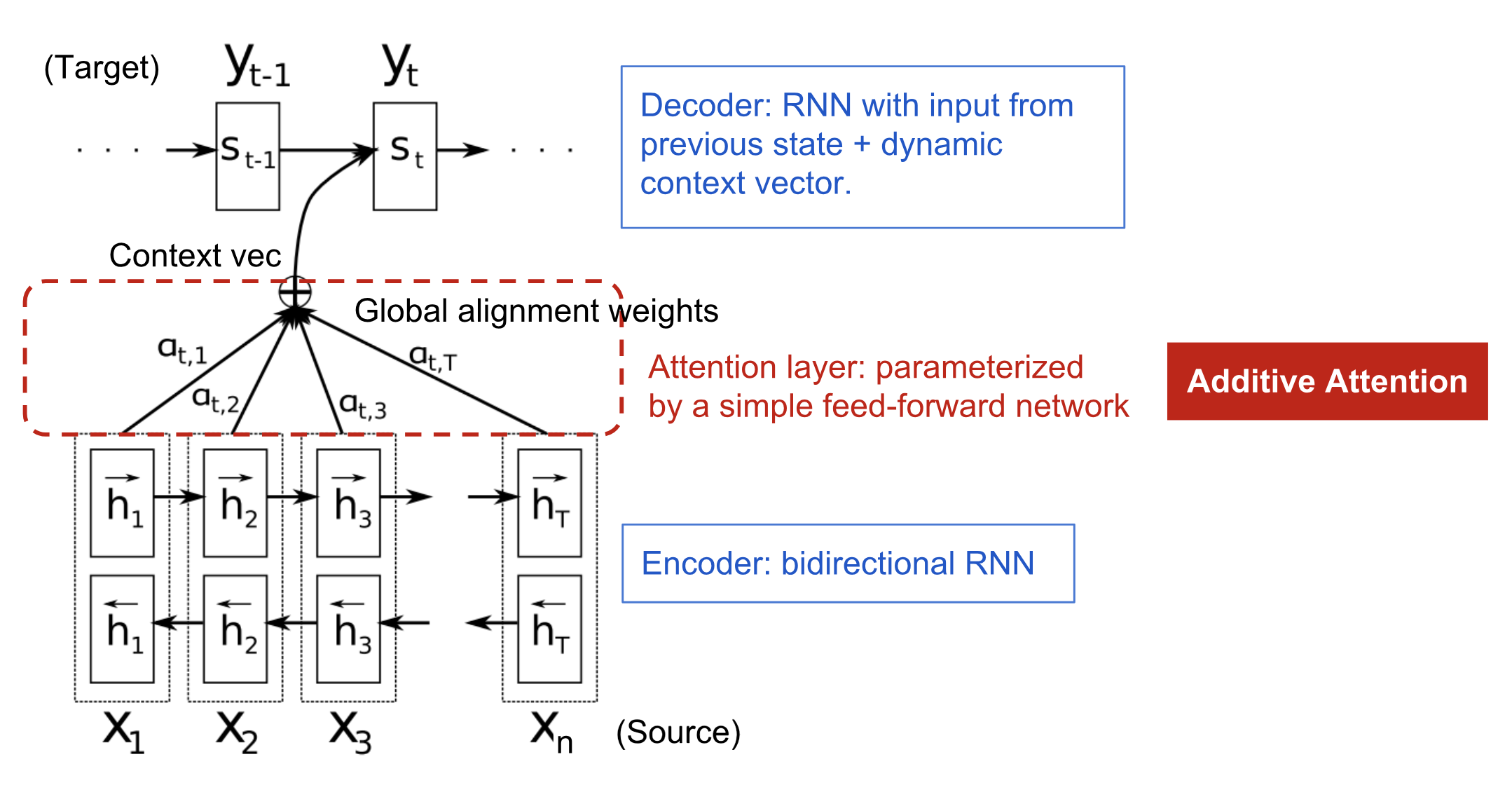
NMT by jointly learning to align and translate (EMNLP 2014)

Encoder

Bi-RNNs, obtain the annotation for each word $x_i$ by concatenating the forward and backward hidden states:

$h_j = [\overrightarrow{h}_j^T, \overleftarrow{h}_{j}^T]^T$

Decoder

The conditional probability is :

$p(y_i|y_1,...,y_{i-1},\mathbf{x}) = g(y_{i-1}, s_i, c_i)$

where $s_i$ is the RNN hidden state for time $i$:

$s_i = f(s_{i-1}, y_{i-1}, c_i)$

Unlike the basic encoder-decoder architecture, the probability of each output word is conditioned on a distinct context vector $c_i$ for each target word $y_i$ .

$c_i = \sum_{j=1}^{T_x} \alpha_{ij} h_j$ $\alpha_{ij} = \frac{\exp(e_{ij})}{\sum_{k=1}^{T_x} \exp(e_{ik})}$ $e_{ij} = score(s_{i-1}, h_j)$

where $e_{ij}$ is an alignment model which scores how well the input at the position $j$ and the output at position $i$ match ^[3]. Here $\text{score}$ is a simple FF-NN layer:

$\text{score}(s_t, \mathbf{h}_i) = \mathbf{v}_a^T \tanh(\mathbf{W}_a[s_t; \mathbf{h}_i])$

where $\mathbf{v}_a$ and $\mathbf{W}_a$ are learnable.

Img source: M. Ji's blog

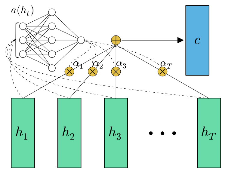
Attention zoo

Content-based location	Alignment score function
Concat (additive, FF_NN)^[5]	$$\text{score}(\mathbf{h}_t, \overline{\mathbf{h}}_s) = \mathbf{v}_a^T \tanh(\mathbf{W}_a [\mathbf{h}_t; \overline{\mathbf{h}}_s] )$$
General ^[5]	$$\text{score}(\mathbf{h}_t, \overline{\mathbf{h}}_s) = \mathbf{h}_t^T \mathbf{W}_a \overline{\mathbf{h}}_s $$
Dot-product ^[5]	$$\text{score}(\mathbf{h}_t, \overline{\mathbf{h}}_s) = \mathbf{h}_t^T \overline{\mathbf{h}}_s$$
Scaled dot-product ^[6]	$$\text{score}(\mathbf{h}_t, \overline{\mathbf{h}}_s) = \frac{ \mathbf{h}_t^T \overline{\mathbf{h}}_s}{\sqrt{d}}$$ where $d$ is the dimension of the source input hidden states.
Self-attention ^[7]	Replace the target sequence with the same input sequence with other attention function.
Location-based attention	Alignment score function
Location-based ^[5]	$$ \alpha_{ij} = \text{softmax}(\mathbf{W}_a \mathbf{h}_{t=j})$$

image source:^[5]

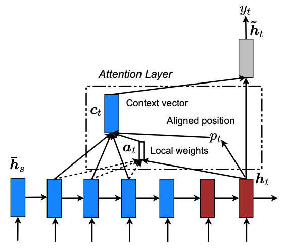
FF-FC attention(a.k.a additive attention)^[9]

Transformer

Background

End2end memory networks are based on a recurrent attention mechanism instead of sequence-aligned recurrence. However, sequence-aligned RNNs preclude parallelization.

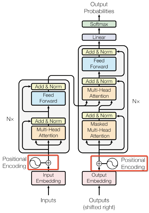
Model architecture

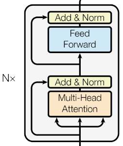
Architecture: stacked self-attention + point-wise FC layer (with residual connection + layer normalization)

Encoder

The transformer encoder applies one multi-head attention followed by one FC-FF layer, adopting the residual connection and layer normalization trick: $\text{LayerNorm}(x+ \text{Sublayer}(x))$

class SublayerConnection(nn.Module):
    """
    a residual connection followed by a layer norm
    """
    def __init__(self, size, dropout):
        super(SublayerConnection, self).__init__()
        self.norm = nn.LayerNorm(size)
        self.dropout = nn.Dropout(dropout)

    def forward(self, x, sublayer):
        """ Apply residual connection to any sublayer with the same size"""
        return x + self.dropout(sublayer(self.norm(x)))

Layer Normalization:

$y = \gamma * \frac{x - E[x]}{\sqrt{\text{Var}[x]+\epsilon}} + \beta$

where $\gamma$ and $\beta$ are learnable affine transform parameters.

class LayerNorm(nn.Module):
    """ layer norm"""

    def __init__(self, size, eps=1e-6):
        super(LayerNorm, self).__init__()
        self.weight = nn.Parameter(torch.ones(size))
        self.bias = nn.Parameter(torch.zeros(size))
        self.eps = eps

    def forward(self, x):
        mean = x.mean(-1, keepdim=True)
        std = x.std(-1, keepdim=True)
        return self.weight * (x - mean) / (std + self.eps) + self.bias

N = 6 stack transformer layers
Output dimension $d_{model}$ = 512

def clones(module, N):
    """ produce N identical layers """
    return nn.ModuleList([copy.deepcopy(module) for _ in range(N)])
    
class Encoder(nn.Module):
    """ Core encoder -> a stack of N layers """
    def __init__(self, layer, N):
        super(Encoder, self).__init__()
        self.layers = clones(layer, N)
        self.norm = nn.LayerNorm(layer.size)

    def forward(self, x, mask):
        """ pass input and mask through each layer in turn"""
        for layer in self.layers:
            x = layer(x, mask)
        return self.norm(x)


class EncoderLayer(nn.Module):
    """ encoder consists of a self-attn and ffc"""

    def __init__(self, size, self_attn, feed_forward, dropout):
        super(EncoderLayer, self).__init__()
        self.self_attn = self_attn
        self.feed_forward = feed_forward
        self.sublayer = utils.clones(SublayerConnection(size, dropout), 2)
        self.size = size

    def forward(self, x, mask):
        x = self.sublayer[0](x, lambda x: self.self_attn(x, x, x, mask))
        return self.sublayer[1](x, self.feed_forward)

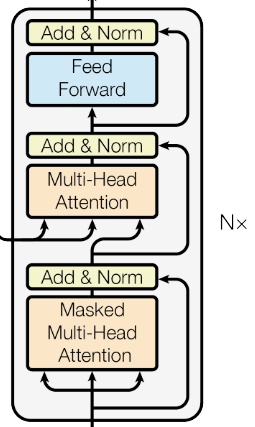
Decoder

Same as the encoder, N = 6 identical stacked layers

class Decoder(nn.Module):
    """ N layer decoder with masking"""
    def __init__(self, layer, N):
        super(Decoder, self).__init__()
        self.layers = clones(layer, N)
        self.norm = nn.LayerNorm(layer.size)

    def forward(self, x, memory, src_mask, tgt_mask):
        for layer in self.layers:
            x = layer(x, memory, src_mask, tgt_mask)
        return self.norm(x)

class DecoderLayer(nn.Module):
    """ decoder"""

    def __init__(self, size, self_attn, src_attn, feed_forward, dropout):
        super(DecoderLayer, self).__init__()
        self.size = size
        self.self_attn = self_attn
        self.src_attn = src_attn
        self.feed_forward = feed_forward
        self.sublyer = utils.clones(SublayerConnection(size, dropout), 3)

    def forward(self, x, memory, src_mask, tgt_mask):
        m = memory
        x = self.sublyer[0](x, lambda x: self.self_attn(x, x, x, tgt_mask))
        x = self.sublyer[1](x, lambda x: self.src_attn(x, m, m, src_mask))
        return self.sublyer[2](x, self.feed_forward)

Difference
The first multi-head attention layer is masked to prevent positions from attending to subsequent positions, ensuring that the prediction output at position $i$ only depends on the known outputs at positions less than $i$, regardless of the future.

def subsequent_mask(size):
    """ Mask out subsequent positions """
    attn_shape = (1, size, size)
    subsequent_mask = np.triu(np.ones(attn_shape), k=1).astype('uint8')
    return torch.from_numpy(subsequent_mask) == 0

Multi-head attention

Transformer regarded encoded representation of input sequences as a set of key-value pairs (K,V), with dimension of input sequence length $n$. In MT context, encoder hidden states serve as (K, V) pairs. In the decoder the previous output is a query (with dimension $m$)

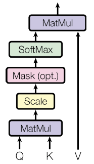
Scaled dot-product attention

$\text{Attention}(\mathbf{Q}, \mathbf{K}, \mathbf{V}) = \text{softmax}(\frac{\mathbf{Q}\mathbf{K}^\top}{\sqrt{d_{k}}})\mathbf{V}$

where $d_k$ is the dimension of the key.

Q: Why dividing $\sqrt{d_{k}}$ in dot-product operation?

For small values of $d_k$ , the additive attention and dopt product attention perform similarly.
For large values of $d_k$ , additive attention outperforms dot product attention without scaling.
Interpretation: The dot products grow large in magnitude, pushing the softmax function into regions where it has extremely small gradients. Assume $q$ and $k$ are independent random variables with mean 0 and variance 1. Their product $q \cdot k = \sum_{i=1}^{d_k} q_i k_i$ has mean 0 and variance $d_k$ . Thus, scales the dot products by $\frac{1}{\sqrt{d_k}}$ .

In conventional attention view:

$\mathbf{h}_t = Q$ $\overline{\mathbf{h}}_s = K = V$ $\text{score}(\mathbf{h}_t, \overline{\mathbf{h}}_s) = \frac{\mathbf{h}_t \overline{\mathbf{h}}_s^T}{\sqrt{d_k}}$ $\alpha_{ij}= \frac{\exp(e_{ij})}{\sum_{k=1}^{d_k} \exp(e_{ik})}$ $c_i = \sum_{j=1}^{d_k} \alpha_{ij} \mathbf{h}_j$

Dot-product is faster and more space-efficient compared with additive attention (one FF layer) in practice.^[6]

More precisely, for the input sequence $x = (x_1, \cdots, x_n)$ , dot-product attention outputs the new sequence $z = (z_1,\cdots, z_n)$ of the same length, $z_i \in \mathbb{R}^{d_z}$

$\begin{align} e_{ij} &= \frac{(x_iW^Q)(x_jW^K)^T}{\sqrt{d_z}}\\ \alpha_{ij} &= \frac{\exp e_{ij}}{\sum_{k=1}^n \exp e_{ik}} \\ z_i &= \sum_{j=1}^n \alpha_{ij} (x_j W^V) \\ \end{align}$

def attention(query, key, value, mask=None, dropout=None):
    """
    scaled dot product
    ---------------------------
    L : target sequence length
    S : source sequence length:
    N : batch size
    
    E : embedding dimension
    h : # of attn head
    d_k: E // h
    ---------------------------
    :param query: (N, h, L, d_k)
    :param key: (N, h, S, d_k)
    :param value: (N, h, S, d_k)
    :param mask:
    :param dropout: float
    :return:
    """
    d_k = query.size(-1)
    # (nbatch, h, seq_len, d_k) @ (nbatch, h, d_k, seq_len) => (nbatch, h, seq_len, seq_len)
    scores = torch.matmul(query, key.transpose(-2, -1)) / math.sqrt(d_k)
    if mask is not None:
        scores = scores.masked_fill(mask == 0, -1e9)
    p_attn = F.softmax(scores, dim=-1)
    if dropout:
        p_attn = dropout(p_attn)
    # (nbatch, h, seq_len, seq_len) @ (nbatch, h, seq_len, d_k) = > (nbatch, h, seq_len, d_k)
    return torch.matmul(p_attn, value), p_attn

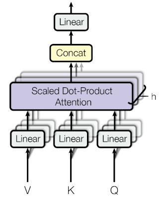
Multi-head attention

Multi-head: “linear project the $Q$, $K$ and $V$ $h$ times with different, learned linear projections to $d_k$ , $d_k$ and $d_v$ dimensions, respectively.”^[6] Then concat all ($h$) the $d_v$ and use a linear layer to project to the final representation values.

Multi-head allows to “jointly attend to information from different representation subspaces at different positions“:

$\begin{align} \text{MultiHead}(\mathbf{Q},\mathbf{K},\mathbf{V}) &= \text{concat}(\text{head}_1,...,\text{head}_h) \mathbf{W}^O \\ \text{head}_i &= \text{Attention}(\mathbf{Q} W_i^Q,\mathbf{K} W_i^K,\mathbf{V}W_i^V) \end{align}$

where $W_i^Q \in \mathbb{R}^{d_{model} \times d_k}$ , $W_i^K \in \mathbb{R}^{d_{model} \times d_k}$ , $W_i^V \in \mathbb{R}^{d_{model} \times d_v}$ , $W_i^O \in \mathbb{R}^{hd_{v} \times d_{model}}$

class MultiHeadedAttention(nn.Module):
    def __init__(self, h, d_model, dropout=0.1):
        """
        multi-head attention
        :param h: nhead
        :param d_model: d_model
        :param dropout: float
        """
        super(MultiHeadedAttention, self).__init__()
        assert d_model % h == 0
        #  split d_model into h heads
        self.d_k = d_model // h
        self.h = h
        self.linears = utils.clones(nn.Linear(d_model, d_model), 4)
        self.attn = None
        self.dropout = nn.Dropout(p=dropout)

    def forward(self, query, key, value, mask=None):
        """
        ---------------------------
        L : target sequence length
        S : source sequence length:
        N : batch size
        E : embedding dim
        ---------------------------
        :param query: (N,L,E)
        :param key: (N,S,E)
        :param value: (N,S,E)
        :param mask: 
        """
        if mask is not None:
            # Same mask applied to all h heads.
            mask = mask.unsqueeze(1)
        nbatches = query.size(0) # batch size

        # 1) split embedding dim to h heads : from d_model => h * d_k
        # dim: (nbatch, h, seq_length, d_model//h)
        query, key, value = \
            [l(x).view(nbatches, -1, self.h, self.d_k).transpose(1, 2)
             for l, x in zip(self.linears, (query, key, value))]

        # 2) compute attention
        x, self.attn = attention(query, key, value, mask=mask, dropout=self.dropout)

        # 3) "Concat" using a view and apply a final linear.
        # dim: (nbatch, h, d_model)
        x = x.transpose(1, 2).contiguous().view(nbatches, -1, self.h * self.d_k)
        return self.linears[-1](x)

Transformer attention:

Mimic the conventional encoder-decoder attention mechanisms: $Q$ comes from previous decoder, $K$, $V$ come from the decoder output. This allows every position in the decoder to attend over all positions in the input sequence (as figure above).
Encoder: K=V=Q, i.e. the output of previous layer. Each position in the encoder can attend to all positions in the previous layer of the encoder.
Decoder: allow each position in the decoder to attend to all positions in the decoder up to and including that position.

Point-wise feed-forward nets

$\text{FFNN}(x) = \max(0, xW_1 + b_1) W_2 + b_2$

class PositionwiseFeedForward(nn.Module):
    """ FFN """
    def __init__(self, d_model, d_ff, dropout=.1):
        super(PositionwiseFeedForward, self).__init__()
        self.w_1 = nn.Linear(d_model, d_ff)
        self.w_2 = nn.Linear(d_ff, d_model)
        self.dropout = nn.Dropout(dropout)

    def forward(self, x):
        return self.w_2(self.dropout(F.relu(self.w_1(x))))

Positional encoding

Drawbacks: self-attention cannot capture the order information of input sequences.

Positional embeddings can be learned or pre-fixed ^[8].

RNNs solution: inherently model the sequential information, but preclude parallelization.

Residual connections help propagate position information to higher layers.

Absolute Positional Encoding

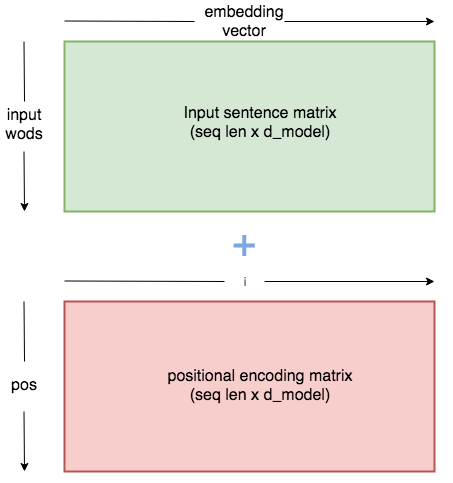
Transformer solution: use sinusoidal timing signal as positional encoding (PE).

$PE_{(\text{pos}, 2i)} = \sin(\frac{\text{pos}}{10000^{2i/d_\text{model}}})$ $PE_{(\text{pos}, 2i+1)} = \cos(\frac{\text{pos}}{10000^{2i/d_\text{model}}})$

where $\text{pos}$ is the position in the sentence and $i$ is the order along the embedding vector dimension. Assume this allows to learn to attend by relative positions, since for and fixed offset $k$, $\text{PE}_{\text{pos}+k}$ can be represented as the linear function of $\text{PE}_{\text{pos}}$ ^[6]

# positional encoding layer in PyTorch
class PositionalEncoding(nn.Module):
    def __init__(self, d_model, dropout, max_len=5000):
        super(PositionalEncoding, self).__init__()
        self.dropout = nn.Dropout(p=dropout)

        pe = torch.zeros(max_len, d_model)
        position = torch.arange(0., max_len).unsqueeze(1) # generate with maximum length
        div_term = torch.exp(torch.arange(0., d_model, 2) * - (math.log(1e4) / d_model))
        pe[:, ::2] = torch.sin(position * div_term)
        pe[:, 1::2] = torch.cos(position * div_term)
        pe = pe.unsqueeze(0)
        self.register_buffer('pe', pe)

    def forward(self, x):
        seq_len = x.size(1) # take the sequence length
        x = x + Variable(self.pe[:, :seq_len], requires_grad=False)
        return self.dropout(x)

Usage: before stacked encoder/decoder, take the sum of PE and input embeddings (as figure below).

class Embeddings(nn.Module):
    def __init__(self, d_model, vocab):
        super(Embeddings, self).__init__()
        self.lut = nn.Embedding(vocab, d_model)
        self.d_model = d_model

    def forward(self, x):
    	"""
        increase the embedding values before addition is to make positional encoding relatively smaller
        """
        return self.lut(x) * math.sqrt(self.d_model)

Relative Positional Representation(RPR)

Relation-aware self-attn
Consider the pairwise relationships between input elements, which can be seen as a labeled, directed fully-connected graph. Let $a_{ij}^V,a_{ij}^K \in \mathbb{R}^{d_a}$ represent the edge between input elements $x_i$ and $x_j$ .

Then add the pairwise information to the sublayer output:

$\begin{align} e_{ij} &= \frac{x_i W^Q (x_j W^K \color{red}{+a_{ij}^K})^\top}{\sqrt{d_z}} \\ &= \frac{x_i W^Q (x_jW^K)^\top + \overbrace{\color{green}{\pmb{x_iW^Q(a_{ij}^K)^\top}}}^\text{efficient implementation}}{\sqrt{d_z}} \\ \alpha_{ij} &= \frac{\exp e_{ij}}{\sum_{k=1}^n \exp e_{ik}} \\ z_i &= \sum_{j=1}^n \alpha_{ij}(x_jW^V \color{red}{+ a_{ij}^V} )\\ \end{align}$

Clip RPR
$k$ denotes the maximum relative position. The relative position information beyond $k$ will be clipped to the maximum value, which generalizes to the unseen sequence lengths during training.^[14] In other words, RPR only considers context in a fixed window size $2k+1$, indicating $k$ elements on the l.h.s, and $k$ elements on the r.h.s, as well as itself.

$\begin{align} \text{clip}(x,k) &= \max(-k, \min(k,x)) \\ a_{ij}^K &= w_{\text{clip}(j-i, k)}^K \\ a_{ij}^V &= w_{\text{clip}(j-i, k)}^V \end{align}$

where rpr $w^K = (w_{-k}^K, \cdots, w_k^K) \in \mathbb{R}^{d_a}$ and $w^V = (w_{-k}^V, \cdots, w_k^V) \in \mathbb{R}^{d_a}$ are learnable.

Trainable param number:

MADPA: $\overbrace{4 \times \big(\text{d_model} \times \text{d_model} + \text{d_model} \big)}^\text{4 dense layers}$
MADPA with RPR: $\underbrace{4 \times \big(\text{d_model} \times \text{d_model} + \text{d_model} \big)}_\text{4 dense layers} + \underbrace{\color{red}{2 \times (\text{seq_len}^2 \times d_k )}}_\text{2 RPR matrices}$

PyTorch implementation

class MultiHeadedAttention_RPR(nn.Module):
    """ @ author: Yekun CHAI """
    def __init__(self, d_model, h, max_relative_position, dropout=.0):
        """
        multi-head attention
        :param h: nhead
        :param d_model: d_model
        :param dropout: float
        """
        super(MultiHeadedAttention_RPR, self).__init__()
        assert d_model % h == 0
        #  assume d_v always equals d_k
        self.d_k = d_model // h
        self.h = h
        self.linears = utils.clones(nn.Linear(d_model, d_model), 4)
        self.dropout = nn.Dropout(p=dropout)

        self.max_relative_position = max_relative_position
        self.vocab_size = max_relative_position * 2 + 1
        self.embed_K = nn.Embedding(self.vocab_size, self.d_k)
        self.embed_V = nn.Embedding(self.vocab_size, self.d_k)

    def forward(self, query, key, value, mask=None):
        """
        ---------------------------
        L : target sequence length
        S : source sequence length:
        N : batch size
        E : embedding dim
        ---------------------------
        :param query: (N,L,E)
        :param key: (N,S,E)
        :param value: (N,S,E)
        :param mask:
        """
        nbatches = query.size(0)  # batch size
        seq_len = query.size(1)
        # 1) split embedding dim to h heads : from d_model => h * d_k
        # dim: (nbatch, h, seq_length, d_model//h)
        query, key, value = \
            [l(x).view(nbatches, -1, self.h, self.d_k).transpose(1, 2)
             for l, x in zip(self.linears, (query, key, value))]

        # 2) rpr
        relation_keys = self.generate_relative_positions_embeddings(seq_len, seq_len, self.embed_K)
        relation_values = self.generate_relative_positions_embeddings(seq_len, seq_len, self.embed_V)
        logits = self._relative_attn_inner(query, key, relation_keys, True)
        weights = self.dropout(F.softmax(logits, -1))
        x = self._relative_attn_inner(weights, value, relation_values, False)
        # 3) "Concat" using a view and apply a final linear.
        # dim: (nbatch, h, d_model)
        x = x.transpose(1, 2).contiguous().view(nbatches, -1, self.h * self.d_k)
        return self.linears[-1](x)

    def _generate_relative_positions_matrix(self, len_q, len_k):
        """
        genetate rpr matrix
        ---------------------------
        :param len_q: seq_len
        :param len_k: seq_len
        :return: rpr matrix, dim: (len_q, len_q)
        """
        assert len_q == len_k
        range_vec_q = range_vec_k = torch.arange(len_q)
        distance_mat = range_vec_k.unsqueeze(0) - range_vec_q.unsqueeze(-1)
        disntance_mat_clipped = torch.clamp(distance_mat, -self.max_relative_position, self.max_relative_position)
        return disntance_mat_clipped + self.max_relative_position

    def generate_relative_positions_embeddings(self, len_q, len_k, embedding_table):
        """
        generate relative position embedding
        ----------------------
        :param len_q:
        :param len_k:
        :return: rpr embedding, dim: (len_q, len_q, d_k)
        """
        relative_position_matrix = self._generate_relative_positions_matrix(len_q, len_k)
        return embedding_table(relative_position_matrix)

    def _relative_attn_inner(self, x, y, z, transpose):
        """
        efficient implementation
        ------------------------
        :param x: 
        :param y: 
        :param z: 
        :param transpose: 
        :return: 
        """
        nbatches = x.size(0)
        heads = x.size(1)
        seq_len = x.size(2)

        # (N, h, s, s)
        xy_matmul = torch.matmul(x, y.transpose(-1, -2) if transpose else y)
        # (s, N, h, d) => (s, N*h, d)
        x_t_v = x.permute(2, 0, 1, 3).contiguous().view(seq_len, nbatches * heads, -1)
        # (s, N*h, d) @ (s, d, s) => (s, N*h, s)
        x_tz_matmul = torch.matmul(x_t_v, z.transpose(-1, -2) if transpose else z)
        # (N, h, s, s)
        x_tz_matmul_v_t = x_tz_matmul.view(seq_len, nbatches, heads, -1).permute(1, 2, 0, 3)
        return xy_matmul + x_tz_matmul_v_t

Tensorflow implementation: ^[16]

Thought: current attention mechanism is one round, and one dimension (at sequence dimension)

Citation

@misc{chai2019attn-summary,
  author = {Chai, Yekun},
  title = {{Attention in a Nutshell}},
  year = {2019},
  howpublished = {\url{http://cyk1337.github.io/notes/2019/01/22/NLP/Attention-in-a-nutshell/}},
}

References

1.Sutskever, I., Vinyals, O., & Le, Q. V. (2014). Sequence to sequence learning with neural networks. In Advances in neural information processing systems (pp. 3104-3112). ↩
2.Weng L. (2018, Jun 24). Attention? Attention! [Blog post]. Retrieved from https://lilianweng.github.io/lil-log/2018/06/24/attention-attention.html ↩
3.Bahdanau, D., Cho, K., & Bengio, Y. (2014). Neural Machine Translation by Jointly Learning to Align and Translate. CoRR, abs/1409.0473. ↩
4.Cho, K., Merrienboer, B.V., Bahdanau, D., & Bengio, Y. (2014). On the Properties of Neural Machine Translation: Encoder-Decoder Approaches. SSST@EMNLP. ↩
5.Luong, T., Pham, H., & Manning, C.D. (2015). Effective Approaches to Attention-based Neural Machine Translation. EMNLP. ↩
6.Vaswani, A., Shazeer, N., Parmar, N., Uszkoreit, J., Jones, L., Gomez, A.N., Kaiser, L., & Polosukhin, I. (2017). Attention Is All You Need. NIPS. ↩
7.Cheng, J., Dong, L., & Lapata, M. (2016). Long Short-Term Memory-Networks for Machine Reading. EMNLP. ↩
8.LeCun, Y., Bottou, L., & Bengio, Y. (2006). PROC OF THE IEEE NOVEMBER Gradient Based Learning Applied to Document Recognition. ↩
9.Raffel, C., & Ellis, D.P. (2015). Feed-Forward Networks with Attention Can Solve Some Long-Term Memory Problems. CoRR, abs/1512.08756. ↩
10.Towards Data Science: How to code the transformer in PyTorch ↩
11.Harvard nlp: the annotated Transformer ↩
12.Illustrated Transformer ↩
13.Medium: How Self-Attention with Relative Position Representations works ↩
14.Shaw, P., Uszkoreit, J., & Vaswani, A. (2018). Self-attention with relative position representations. arXiv preprint arXiv:1803.02155. ↩
15.RPR blog (in Chinese) ↩
16.Tensor2Tensor tensorflow code ↩
17.Attn: Illustrated Attention ↩