Text classification is one of the most important fundamental NLP tasks. Its goal is to assign labels to texts, including sentiment analysis, spam detection, topic labeling, Twitter hashtag prediction, domain detection, etc.
Sentence classfication
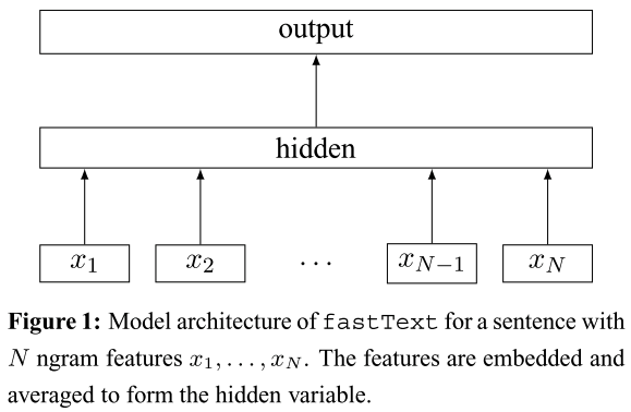
Fasttext (Facebook 2016)
A simple and efficient baseline for text classification.
- Model: average word representations into a text representation, and then feed into a linear classifier (the model architecture is similar to the CBOW model, by replacing the middle word with a label).
- Hierarchical softmax
- N-gram features: Besides bag-of-word features,
bag of n-gramsas additional features to capture partial information about the local word order.
Hashing trick
TextCNN (Kim 2014)
Background
- sparse, 1-of-V encoding low dimensional vector space
CNNs utilize layers with convolving filters that are applied to loca l features. (Lecun et al., 1998) [3]
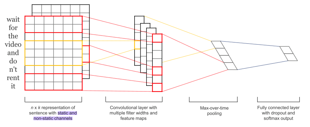
Let be the $k$-dimensional word vectors w.r.t. $i$-th word in the sentence. A sentence with length $n$ (padded if necessary) is:
Convolution op applies filters $\mathbf{w} \in \mathbb{R}^{hk}$ to a window of $h$ words to extract new features:
where $b \in \mathbb{R} $ is a bias term and $f$ is a non-linear function, e.g. hyperbolic tangent.
Thus, for a sentence , generate a feature map $\mathbf{c} \in \mathbb{R}^{n-h+1} $:
Then apply a max-over-time pooling op over the feature map and takes the maximum value as the feature w.r.t. this filter.
max-over-time pooling op is to capture the most important feature - with maximum value - for each feature map.
One feature is extracted from $one$ filter.
TextCNNs use multiple filters with varying window sizes $h$ to get multiple features. Then pass these features to a FC-softmax layer, and output the probability distribution over labels.
Tricks:
- Dropout regularization: prevent co-adaptation of hidden units by randomly dropping out a proportion $p$ of the hidden units during the training process.
Given $\mathbf{c}$, conventional FC layer is:While dropout is:where $ \circ $ is the element-wise multiplication op and $\mathbf{r} \in \mathbb{R}^m$ is a masking vector of Bernoulli random variables with probability $p$ to keep.
At training time, after masking $(1-p)\%$ hidden units, backprop only goes though unmasked units.
At test time, the learned weight $\mathbf{w}$ is scaled by $p$: $\hat{\mathbf{w}} = p \mathbf{w}$. Then $\hat{\mathbf{w}}$ is used at test time without dropout op.
- Weight decay (L2-norm)
TextCNN variants:
- CNN-rand: randomly initialize word vectors during training.
- CNN-static: use pretrained embeddings and keep them static during training, i.e. only train parameters not in embedding layers.
- CNN-non-static: use pretrained embeddings and fine tune, a.k.a. domain-specific training.
- CNN-multichannel: combine aforementioned two scenarios, i.e. use two channels of word embeddings followed by convolution op, but the gradients only backprop through the fine-tuned channel.
Intuition: multichannel CNNs could pervent overfitting (preventing the shift of fine-tuned embeddings by considering original static embeddings in the other channel at the same time), especially on small-scale datasets.
(But results are mixed; further work: on regularizing the fine-tuning process, e.g. use extra dimensions for fine-tune channel)
Static v.s. Non-static representations:
Static: W2V
“good” is similar to “bad” using word2vec!
Because of syntactically equivalenceNon-static: e.g. good ~ nice
Fine-tuning can learn more meaningful representations
Empirical findings on textCNNs:
- Dense pretrained word representations are better than 1-of-V encodings, although different representations perform variously on different tasks.
- Filter rigion size and # of feature maps have a large impact on performance.
- Regularization (dropout or $l2$-norm) has relatively little effect on performance.
Fine-tuning on textCNN suggestions:
- Use non-static word representations instead of one-hot.
- Line-search over the single region size (rather than combined region sizes, e.g. [3,4,5]) to find the best one (e.g. 1~10).
- Alter the # of feature maps for each filter size (from 100~600), with small dropout rate (0-0.5) and large l2-norm constraint.
- Consider different activation functions if possible (ReLU, tanh)
Give a detailed figure of a binary classification task[5]

RCNN (AAAI 2015)
Background
- Recurrent NNs are better to capture the contextual information without the limitation of window size. But it is a biased model since the latter words play more important roles than former contexts.
- ConvNets are unbiased since it can fairly tackle the words in a fixed context with a max-pooling layer. However, it is limited by the pre-defined filter region size. Higher order window size or n-gram could lead to sparse problems.
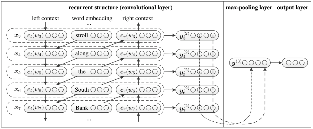
Recurrent ConvNets(RCNN) combines both of them.[6]
Two steps
a) Word representation with recurrent connection
Combine current word embedding and its left and right context (i.e. ) to represent $i$-th word :
Here compute the left and right context representation recursively:
where $f$ is a non-linear activation function.
Afterwards, go through a FC layer with $\tanh$ activation function.
where is a learned word representation, i.e. latent semantic vector.
b) Text representation learning
CNNs are used for text representation. Previous step can be seen as a recurrent convolution op.
Then apply a max-pooling layer:
where $k$-th element of $\mathbf{y}^{(3)}$ is the maximum of the $k$-th elements of $\mathbf{y}_i^{(2)}$.
Finally, go to a FC-softmax layer.
DMN (ICML 2016)
DMN (Dynamic Memory Network)
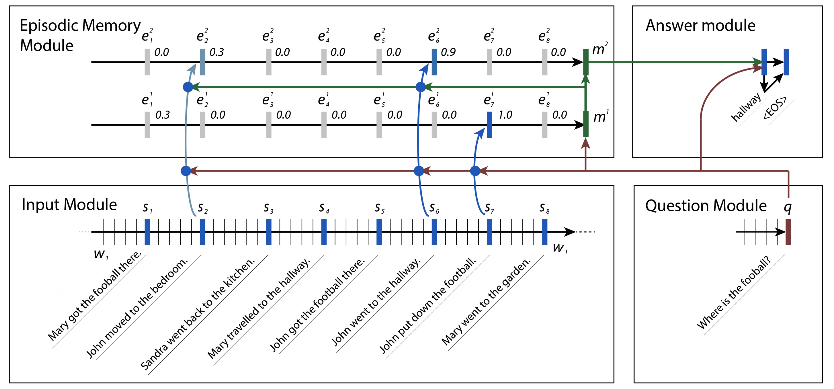
Inituition: Most NLP tasks can be cast as question-answering problems, (e.g. machine translation, sequence modeliing, classification problems) using raw input-question-answer triplets: firstly obtain representations for inputs and the question. The question representation will trigger the iterative attention process by searching at inputs and relevant facts. Then the memory module produces a vector representation of all relevant information to answer the module.
Input module
- Encode raw texts into distributed representations:where $E$ is the embedding lookup table, is the word index of $t$-th word of the input sentence.
Question module
- Encode question into distributed representations with GRU. Unlike input module, output the last hiddden states $q$.
Episodic memory module
- During each iteration, the attention mechanism attends over all the fact representation $c$ with gated function, whilst taking into account the question representation $q$ and the previous memory $m^{i-1}$ to produce the episode $e^i$.
Use gating function as the attention for each pass $i$: $G_i^t = G(c_t, m^{i-1}, q)$.
The scoring function $G$ takes (candidate fact $c$, previous memory $m$, question $q$) as the input feature and output a scala score:where $\circ$ is an element-wise product.
The scoring function is a two-layer FC layer:Memory update: for pass $i$, given a sentence of , the hidden states at time $t$ and episode $e^i$:
Answer module
- Employ another GRU whose initial state is last memory: . At each time, considering the question $q$, last hidden state , as well as previous predicted output .where concat last generated output and question vector .
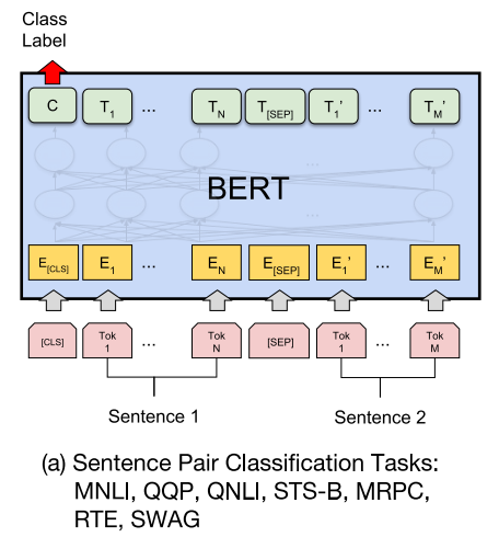
BERT (Google 2018)
Bi-directional Encoder Representations from Transformers
- Model: bi-transformer
- Pretraining:
- Masked Language Models
- Next Sentence Prediction
- Fine-tuning
My solution: github
Document classification
HAN (NAACL 2016)
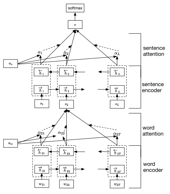
HAN(Hierarchical Attention Net) models the attention mechanism in two levels: word and sentence-level. [4]
- Intuition: incorporating knowledge of document structure in the model architecture.
Because not all parts of documents are equally relevant, and determing the relevant parts includes modeling the interaction of the words, not just their presence in isolation. - Hierarchical structure: words form sentences, sentences form a document.
- Different words and sentences in a document are differently informative. The importance of the informative words and sentences are highly context-dependent.
- Attention mechanism could provide insight into which words and sentences contribute more or less to the decision[4] (by plotting hotmap I think;) )
Architecture
Overall:
- Word-level: a word encoder + word-level attention layer;
- Sentence-level: a sentence encoder + sentence-level attention layer.
Sequence encoder: GRU
Hierarchical attention
Word Encoder
Get word representations from characters using bi-GRU.
Given a sentence with words $w_{it}, t \in [1,T]$, firstly map the words to vectors through an embedding matrix :
Then concat the bi-GRU representation:
HAN[4] directly applied word embeddings for simplification.
Word Attention
Intuition: not all words contribute equally to the sentence representation. Hence employ attention to extract the important words that are most informative and aggregate all the words according to their informativeness (attention vector distribution) to obtain the sentence vector .
Interpretation: firstly feed the word representation into a FC layer to get a hidden representation of . Then measure the (cosine) similarity between the current representation and randomly initialized context , followed by a softmax to obtain the normalized attention weights . Finally, aggregate all the word representations according to the weight vector.
Here, the word context vector is randomly initialized and joint learned during the training process[4]. “The context vector can be seen as a high level representation of a fixed query “what is the informative word” over the words like that used in memory networks.”
Sentence Encoder
Given sentene vector , we get the document vector with bi-GRU (same as word encoder):
Sentence Attention
Same as word attention. Obtain the document vector $v$:
where is sentence-level randomly-initialized sentence context vector, and is joinly learned during training.
Document classification
Feed high-level document representation $v$ into a FC-softmax layer.
The loss function is NLL(negative log likelihood):
where $j$ is the label of the document $d$.
References
- 1.Joulin, A., Grave, E., Bojanowski, P., & Mikolov, T. (2016). Bag of tricks for efficient text classification. arXiv preprint arXiv:1607.01759. ↩
- 2.Devlin, J., Chang, M. W., Lee, K., & Toutanova, K. (2018). Bert: Pre-training of deep bidirectional transformers for language understanding. arXiv preprint arXiv:1810.04805. ↩
- 3.Kim, Y. (2014). Convolutional neural networks for sentence classification. arXiv preprint arXiv:1408.5882. ↩
- 4.Yang, Z., Yang, D., Dyer, C., He, X., Smola, A., & Hovy, E. (2016). Hierarchical attention networks for document classification. In Proceedings of the 2016 Conference of the North American Chapter of the Association for Computational Linguistics: Human Language Technologies (pp. 1480-1489). ↩
- 5.Zhang, Y., & Wallace, B. (2015). A sensitivity analysis of (and practitioners' guide to) convolutional neural networks for sentence classification. arXiv preprint arXiv:1510.03820. ↩
- 6.Lai, S., Xu, L., Liu, K., & Zhao, J. (2015, January). Recurrent Convolutional Neural Networks for Text Classification. In AAAI (Vol. 333, pp. 2267-2273). ↩
- 7.Kumar, A., Irsoy, O., Su, J., Bradbury, J., English, R., Pierce, B., Ondruska, P., Gulrajani, I., & Socher, R. (2016). Ask Me Anything: Dynamic Memory Networks for Natural Language Processing. ICML. ↩
