Embedding Pretrained Linguistic Prior in a Nutshell

Pretraining on ImageNet followed by domain-specific fine-tuning has illustrated compelling improvements in computer vision research. Similarly, Natual Language Processing (NLP) tasks could borrow ideas from this.

Employing pretrained word representations or even langugage models to introduce linguistic prior knowledge has been common sense in amounts of NLP tasks with deep learning.

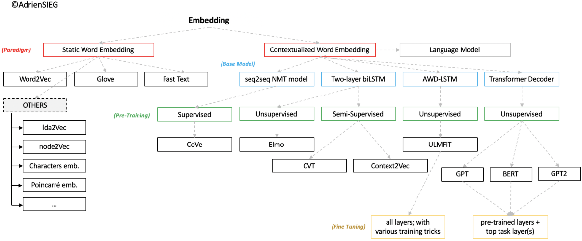
Background

Language Model (LM)

Probability of a sequence of words.
Goal: learn the joint probability function of sequences of words in a language $\prod_{i=1}^N P(w_i | w_{1},..., w_{i-1})$

Challenge: the curse of dimensionality

Discrete n-gram

For a sentence S of length n: $w_1,...,w_m$:

$$P(S) = P(w_1,...,w_n) = \prod_{i=1}^m P(w_i|w_0,...,w_{i-1}) \\ \approx \prod_{i=1}^n \underbrace{P(w_i|w_{i-1},...,w_{i-n+1})}_\textrm{Markov assumption}$$

Strong Markov assumption: for each word i, the probability only depends on previous n-1 words:

• zerogram: uniform distribution
• unigram: word frenquency
• bigram: $x_i$ depends only on $x_{i-1}$
• trigram: $x_i$ depends only on $x_{i-2}, x_{i-1}$

n-gram models:

$$P(w_i|w_1,w_2,...,w_{i-1}) \approx P(w_i | w_{i-(n-1)},...,w_{i-1})$$

MLE by counting:

$$P(w_i | w_{i-(n-1)},...,w_{i-1}) = \frac{ \text{count}(w_{i-(n-1)},...,w_{i-1}) }{ \text{count}(w_{i-(n-1)},...,w_{i}) }$$

Problems: cound-based methods cannot deal with out-of-vocabulary (OOV, i.e. unseen words )

Solution: smoothing (discounting)
Core idea: reserve part of probability mass for unseen events.

Methods:

• Add-1 smoothing (Laplace smoothing)
• Add-$\alpha$ smoothing
• Stupid backoff
• Interpolation
• Kneser-Ney smoothing

Continuous n-gram

Rather than discounting, rely on similarity in internal representation for estimating unseen events.

Relationship between LM and word representation (personal thoughts): neural network(NN) is another way to do matrix factorization but with non-linear transformation. LMs aims to learn the joint distribution function of word sequences, which accumulates conditional probability word by word. Before passing the softmax for normalization, the compact projection layer hidden states could provide effective insights to tell the difference among vocabularies (after softmax normalization). As the subsidiary product of LMs, low dimensional projection states could mitigate the curse of dimensionality and serve for NLP transfer learning.

The earliest idea using NN for LM is not (Bengio et al., 2003). Previous work e.g. (Miikkulainen and Dyer, 1991).

NNLM (Bengio et al., 2003)

Employed NN in statistical n-gram LM.

Learns simultaneously

1. Distributed representation (see following section for details) for each word;
2. Joint probability function $f(w_t,w_{t-1},...,w_{t-n+1})$ for word sequences.

• Input: n-1 context words
• Output: probability distribution of the next word
• Model: a linear projection layer + a non-linear hidden layer. 1 non-linear hidden layer beyond the word feature mapping (i.e. embedding lookup). Optionally, direct feed lookup word vectors to final layer (Implicitly ResNets!). When the hidden states W is set to 0, there is no direct connection.
• Parameter set: $\Theta = (C, \omega)$, where C is word vector mapping, $\omega$ denotes parameters.
• Loss function:
  $L=\frac{1}{T} \sum_t log f(w_t,w_{t-1},...,w_{t-n+1};\Theta) + R(\Theta)$, where $R(\Theta)$ is a regularization term.

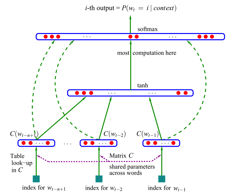
As below figure, NNLMs decompose the n-gram joint probabilty function $f(w_t,...,w_{t-n+1}) = \hat{P}(w_t|w_1^{t-1})$:

1. Mapping matrix C with dimension $ |V| \times m $, represents the distributed feature vector associated with each word in the vocabulary (embedding matrix, a.k.a embedding loopup table).
2. probability function over words: $$f(w_t,w_{t-1},...,w_{t-n+1}) = g(i, C(w_{t-1}),...,C(w_{t-n+1}))$$ where C(i) is the i-th word feature vector.

Solved issue: OOV

Drawbacks:

1. Limited context length (fixed n) that needs to be specified ad hoc before training, only consider previous n-1 words;
2. Simple NN architecture;
3. Word feature representation (embedding) cannot deal with polysemy, which assign each word a single point in a continuous semantic space. Proposed future solution: assign each word sense with different points.

RNNLM (Mikolov et al., 2010)

NNLMs utilize fixed context length which needs to be pre-specified. RNNLMs encode temporal information implicitly for contexts with arbitrary lengths.

• Motivation: condition on arbitrarily long context $\rightarrow$ no Markov assumption
• Input: 1-of-K encoding over the vocabulary with size |V|
• Read in one word at a time, and update hidden state incrementally;
• Hidden state is initialized as empty vectors at time step 0;
• Parameters
  • Embedding matrix $E$
  • Feedforward matrices $W_1$, $W_2$
  • Recurrent maxtrix $U$
• Training: BPTT

Simple RNNs:

$$h_i=\left\{ \begin{array}{ll} 0, \quad if \ i = 0\\ \tanh( W_1Ex_i + Uh_{i-1} ), if\ i > 0\quad \end{array} \right.$$ $$y_i = \text{softmax} (W_2 h_{i-1})$$

Basic LSTM RNNs:

$$\left[\begin{array}{c} \mathbf{i}^c_j\\ \mathbf{o}^c_j \\ \mathbf{f}^c_j \\ \tilde{c}^c_j \end{array}\right] = \left[\begin{array}{c} \sigma \\ \sigma \\ \sigma \\ \tanh \end{array}\right] (\mathbf{W}^{c^T} \left[\begin{array}{c} \mathbf{x}^c_j \\ \mathbf{h}^c_{j-1}\end{array}\right] + \mathbf{b}^c)$$ $$\mathbf{c}^c_j = \mathbf{f}^c_j \odot \mathbf{c}^c_{j-1} + \mathbf{i}^c_j \odot \tilde{c}^c_{j}$$ $$\mathbf{h}_j^c = \mathbf{o}_j^c \odot \tanh(\mathbf{c}^c_j)$$

where $\mathbf{i}^c_j$, $\mathbf{f}^c_j$, $\mathbf{o}^c_j$ denotes a set of input, forget and output gates, respectively. $\mathbf{c}^c_j$ denotes the char cell vector, $\mathbf{h}^c_j$ denotes the hidden vector on each char $c_j$, $\mathbf{W}^{c^T}$, $\mathbf{b}^c$ are parameters.

---

Intrinsic evaluation of LM

Perplexity (PP):

Intuitional interpretation: weighted average branching factor

$$\begin{aligned}PP (S) &{}= P(w_1,...,w_N) = P(w_1,w_2,...,w_N)^{-\frac{1}{N}} \\ &{}= \sqrt[N]{\frac{1}{P(w_1w_2...w_N)}} \\ &{}= \sqrt[N]{\prod_{i=1}^N\frac{1}{P(w_i|w_1...w_{i-1})}}\end{aligned}$$

For bigram models:

$$PP (S) = \sqrt[N]{\prod_{i=1}^N\frac{1}{P(w_i|w_{i-1})}}$$

---

LM application

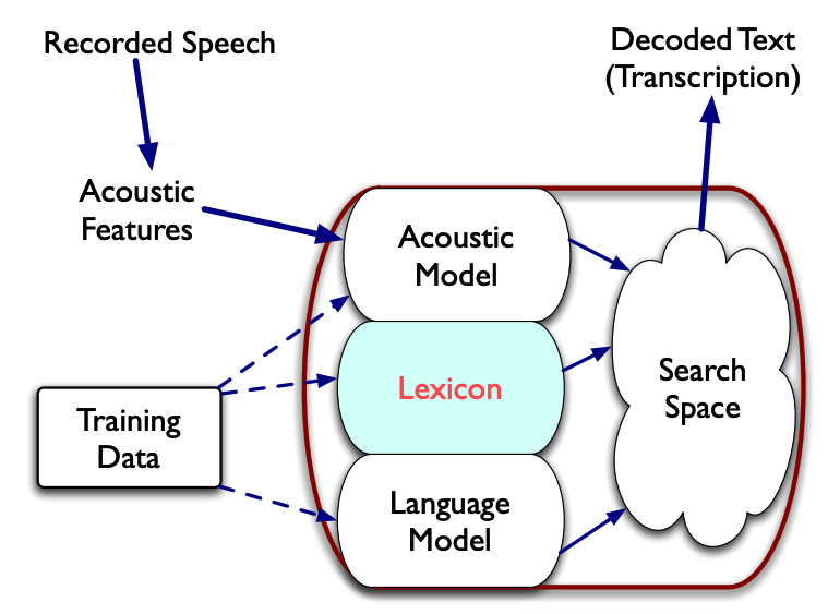
LMs serve as a component in various NLP tasks, such as ASR, MT.

Automatic Speech Recognition

Image source: Steve Renals, Edinburgh Informatics (INFR11033)

Machine Translation

Let T denote a target sentence of length m :$x_1, ..., x_m$, S denote a source sentence n: $y_1,...,y_n$. The machine translation can be expressed as:

$$T^* = \arg\max_T P(T|S) \\= \arg\max_T P(y_1,...,y_n|x_1,...,x_m) \\= \prod_{i=1}^n P(y_i | y_{1}, ...,y_{i-1}, x_1,...,x_m)$$

With Bayes’ theorem, we can get:

$$T^* = \arg\max_T P(S|T) \underbrace{P(T)}_{\text{LM}}$$

Word representation

Distributional representation

distributional hypothesis: linguistic items with similar distributions have similar meanings

• Statistical (count-based) method;
• high-dimensional vector representation obtained from the rows of the word-context co-occurrence matrix, whose dimension size equals to the vocabulary size of the corpus.

Approaches:

• One-hot encoding (a.k.a 1-of-K encoding)
• TF-IDF (Term Frequency - Inverse Document Frequency)
  N $\rightarrow$ # of ducuments, $df_t$ $\rightarrow$ Term frequency for term $t$, $d$ $\rightarrow$ document. $$\text{tf}_{t,d} = 1 + \log_{10} \text{count} (t,d) \quad \text{if count} (t,d)>0, \text{ else } 0$$ $$\text{idf}_{t} = \log (\frac{N}{\text{df}_t})$$ $$w_{t,d} = \text{tf}_{t,d} \times \text{idf}_{t}$$
• PPMI
  PMI association between a target word w and a context word c is: $$\text{PMI}(w,c) = \log_2 \frac{P(w,c)}{P(w)P(c)}$$

$$\text{PPMI} = \max(PMI(w,c), 0)$$

PMI: The numerator tells us how often we observed the two words together (assuming we compute probability by using the MLE). The denominator tells us how often we would expect the two words to co-occur assuming they each occurred independently, so their probabilities could just be multiplied. Thus, the ratio gives us an estimate of how much more the target and feature co-occur than we expect by chance.

Distributed (static) word representation

Distributed representations of words in a vector space have become an effective way to capturing fine-grained linguistic regularities.

low-dimensional, dense, compact vector representation.

• NN-based model (such as word2vec, Collobert and Weston embeddings, HLBL embeddings) ,
• Matrix factorization based model on the word-context co-occurrence matrix (such as the Glove from Stanford using direct matrix factorization, the Latent Semantic Analysis using SVD factorization).

You shall know a word by the company it keeps (John Rupert Firth, 1957).

Learning word representations using Language modeling. (Dr. Adam Lopez’s 2018 lecture)

Inherent limitation of word representations:

• indifference to word order and inability to represent idiomatic phrases.
• cannot tackle polysemy

Word2Vec (Mikolov 2013; Google)

Issue
NLP systems treat words as atomic units: map words to the indices in the vocabulary, not considering similarity between words.

• Pros: simplicity, rebustness, simple models
• Cons: require huge amount of data, which is unrealistic in some occasions, e.g. ASR and NMT.

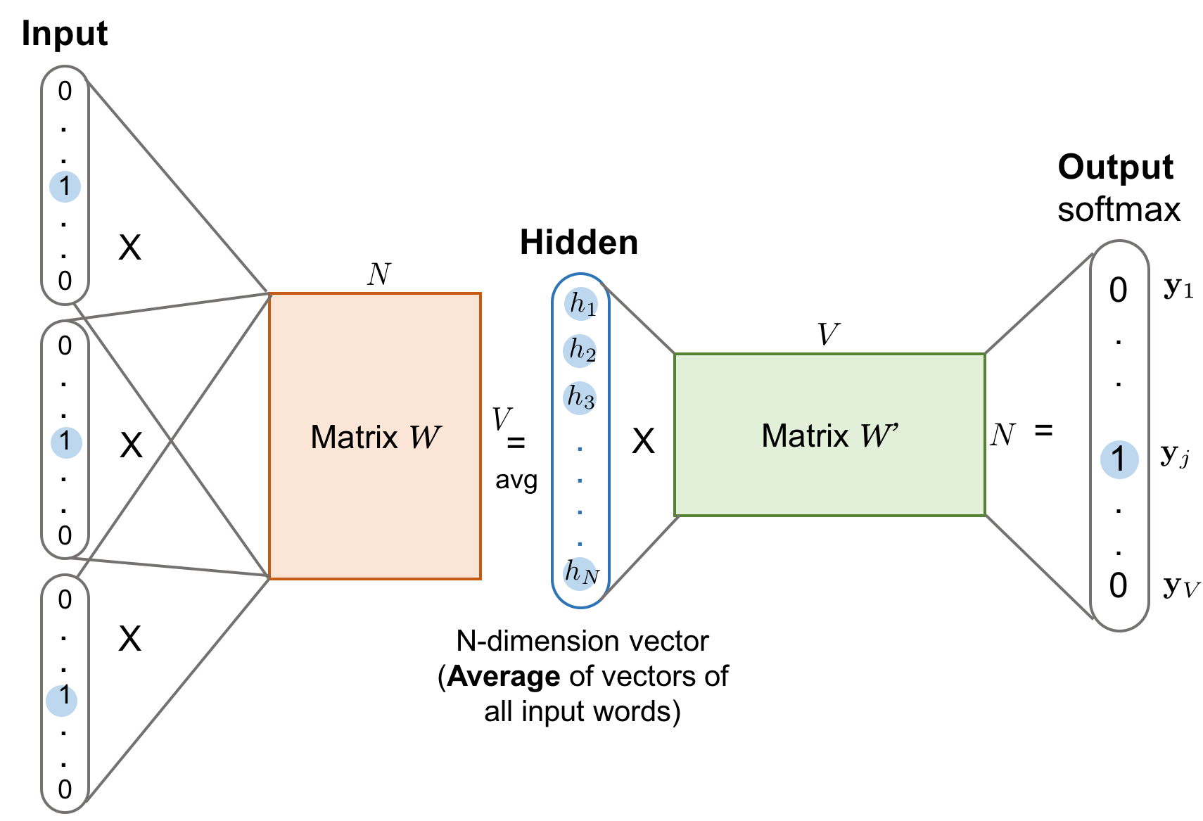
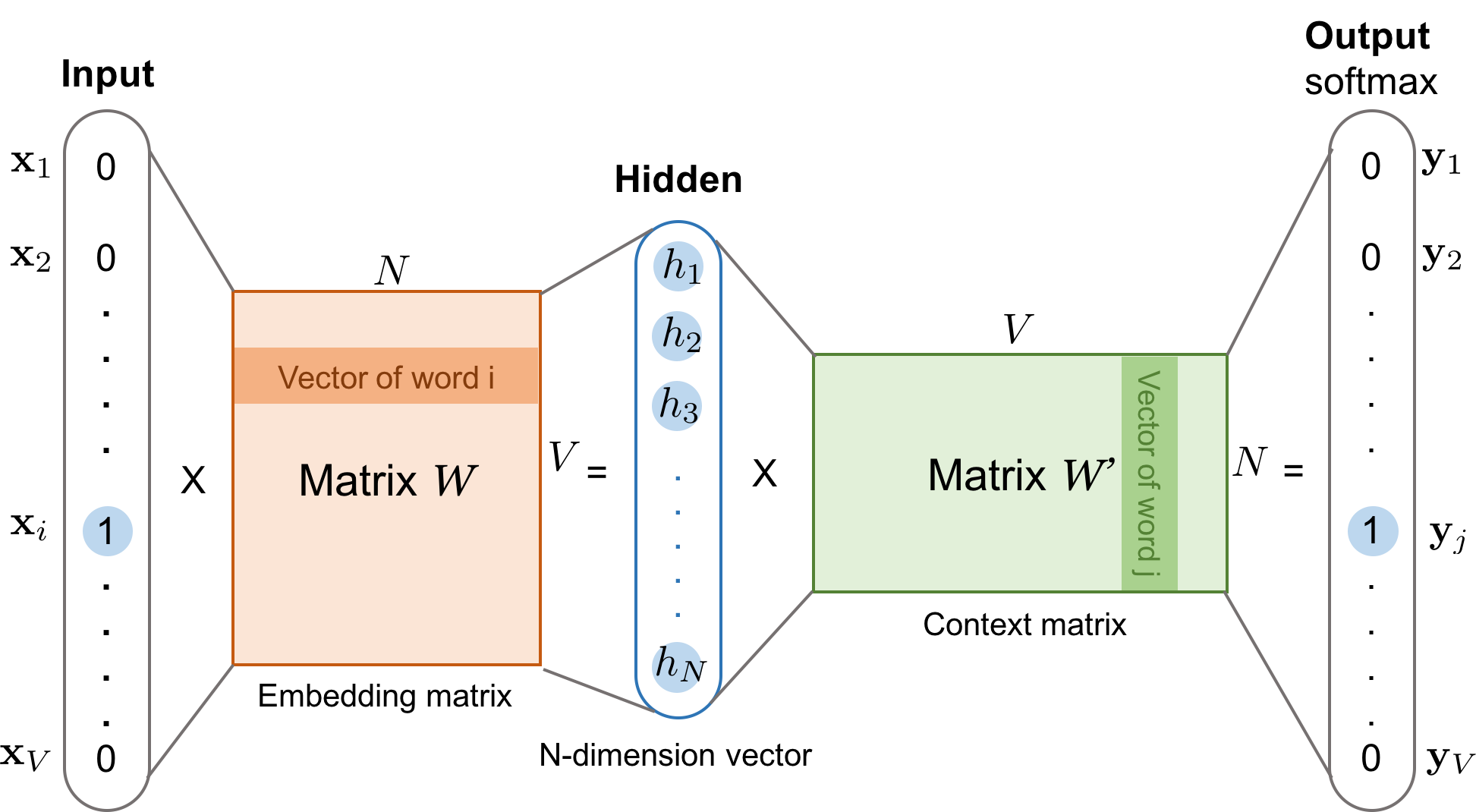
Continuous Bag of Words (CBOW)

• Intuition: predicting the current word based on its context.
• Archtecture: linear projection layer. Feedforward NNLM remove the non-linear hidden layer.
• All words get projected into the same position (vectors are averaged). Called bag-of-word model since the word order in the history doesnot influence the projection.
• Same as NNLMs, weights for different positions are shared.
• Computationally much more efficient than NNLMs.

CBOW ^[9]

Skip-gram

• Intuition: “maximize classification of a word based on another word in the same sentence”, i.e. input each current word to a log-linear classifier with continuous projection layer, and predict words within a certain range before and after the current word.
• Objective: maximize the average log probability, with context size c: $$\frac{1}{T} \sum_{t=1}^T \sum_{-c \leq j \leq c, j \neq 0} \log p(w_{t+j}|w_t)$$
• Simple vector addition can often produce meaningful results. e.g. vec(“Russia”) + vec(“river”) is close to vec(“Volga River”), and vec(“Germany”) + vec(“capital”) is close to vec(“Berlin”).
• Find word representations useful for predicting surrounding words in a sentence or documentation

SkipGram ^[9]

• Issue 1: Inability to represent idiomatic phrases that are not compositions of the individual words.

• Solution: Find out the phrases and treat the phrases as individual tokens during training. Typical analogy pair: vec(“Montreal Canadiens”) - vec(“Montreal”) + vec(“Toronto”) is vec(“Toronto Maple Leafs”).

• Issue 2: very large dimension in softmax layer (size equals to vocabulary size |V|)

• Solution:
  Hierarchical softmax (Morin and Bengio, 2005),
  Negative sampling (NEG) (Mikolov et al. 2013)

Basic softmax (impractical due to computing $\nabla log p(w_O|w_I)$ cost $\propto$ W (~ $10^5 - 10^7$ terms) ):

$$p(w_O|w_I) = \frac{\exp( {v'}_{WO}^T v_{WI} )}{\sum_{w=1}^W \exp({v'}_{W}^T v_{WI})}$$

where $v_w$ and ${v’}_w$ are input and output vector representations of w, W is the vocabulary size.

• Solution 1 $\rightarrow$ Hierarchical softmax
  Instead of computing vocabulary size output nodes in NNs, only need to evaluate ~ $log_2(W)$ nodes.
  (Binary Huffman tree structure)

• Solution 2 $\rightarrow$ Negative sampling: Noise Contrastive Estimation (NCE)
  Differentiate data from noise by means of logistic regression classifier (Gutmann and Hyvärinen, 2010).

Distributed representations capture syntactic and semantic information.

Additional word2vec limitations:

closed vocabulary assumption
cannot exploit functional relationships in learning 

FastText (Mikolov et al. 2017; Facebook)

Issue: Popular models ignores the mophology of words, by assigning distinct vector to each word. Previous popular models ignore the internal structure of words, which is an important limitation for morphologically rich languages, such as Turkish, Finnish.

Bag-of-words $\rightarrow$ Bag of features

Fasttext solution: employ the sum of bag of character n-grams as well as itself for each word, as an extension of skip-gram models. Taking into account subword information.

Let < and > denote the beginning and ending of tokens to distinguish prefixes and suffixes from other character sequences. Taking <where> for example, we use char trigram(n=3), we can get:

char trigram: <wh, whe, her, ere, re>
itself: <where>

Fasttext represents a word by the sum of the vector representations of its n-grams.
Let vector representation $\mathbf{z}_g$ to each n-gram $g$ ($g \in G$) The scoring function:

$$s(w,c) = \sum_{g \in \mathbf{G}} \mathbf{z}_g^T \mathbf{v}_c$$

GloVe (Pennington 2014; Stanford)

GloVe^[8] leverages statistical information by training only on the nonzero elements in a word-word co-occurrence matrix.

Define the co-occurence probability as:

$$p_{\text{co}}(w_k \vert w_i) = \frac{C(w_i, w_k)}{C(w_i)}$$

Intuition: the word meanings are captured by the ratios of co-occurrence probabilities rather than the probabilities themselves. The global vector models the relationship between words i,j towards the thrid context word k:

$$F(w_i, w_j, \tilde{w}_k) = \frac{p_{\text{co}}(\tilde{w}_k \vert w_i)}{p_{\text{co}}(\tilde{w}_k \vert w_j)}$$

For words k like water or fashion, that are either related to both ice and steam, or to neither, the ratio should be close to one.

• build word-word co-occurrence matrix
• do global matrix factorization

---

Challenge

• polysemy
  Frozen representations, can not express polysemy.

• For languages where tokens are not delimited, such as Chinese and Japanese, NLP pipelines require word segmentation ahead. As we know, error generated by upstream tasks would amplified during the following propagation process. Hence, the performance of Chinese word segmentation also counts.

Pretraining (dynamic word representation)

NLP’s ImageNet moment has arrived^[10]
“At the core of the recent advances of ULMFiT, ELMo, and the OpenAI transformer is one key paradigm shift: going from just initializing the first layer of our models to pretraining the entire model with hierarchical representations. If learning word vectors is like only learning edges, these approaches are like learning the full hierarchy of features, from edges to shapes to high-level semantic concepts.”

CV: “Interestingly, pretraining entire models to learn both low and high level features has been practiced for years by the computer vision (CV) community.”

Feature-based pretraining (frozen representation)

ULMFiT

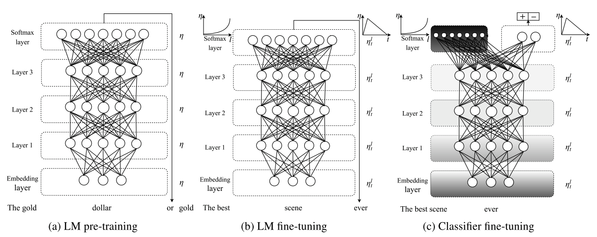
ULMFiT: Universal Language Model Fine-tuning

Problem: LMs overfit to small datasets and suffered catastrophic forgetting when fine-tuned with a classifier.

Solution

• Inductive transfer learning.
• Model: AWD-LSTM ^[19], a regular LSTM (without attention, shot-cut connections)

Three stages:

• General domain LM pretraining
  To capture the general features of the language in different layers;
• Target task LM fine-tuning
  • Trick: discriminative fine-tuning, slanted triangular learning rates
• Target task classifier fine-tuning
  • Trick: concat pooling, gradual unfreezing

Sloved issue

prevent catastrophic forgetting and enable robust transfer learning.

ELMo (NAACL 2018, AllenAI)

Problems

Some word representations are context-independent, only model complex charateristics of word use (e.g. syntax and semantics), ignoring how these uses vary across linguistic context (i.e. polysemy).

Previous improvement:

• Enriching with subword information ^{[15] [7]}
• Learning separate vectors for each word sense ^[16] (as suggested in the conclusion section in the NNLM paper^[1])

Solved issue:

• Seamlessly incorporate multi-sense information into downstream tasks without explicitly training to predefined sense classes.

Solution

• ELMo (Embeddings from Language Models) models polysemy by extracting context-sensitive features.
• Elmo representations are deep $\rightarrow$ a function of all of the internal layers of the biLM.
• Also incorporate subword information, using char ConvNets in the input and output.
• Learn a linear combination of the vectors above each input word. This manner allows for very rich word representations.
• Computing on top of two-layer biLMs with char ConvNets, as a linear function of internal network states.
• After pretrainining the biLM with unlabeled data, ELMo fixes the weights and add additional task-specific model.

High-level LSTM states capture context-dependent aspects of word meaning (perform well on WSD tasks), while lower-level states model aspects of syntax (POS tagging). Simultaneously exposing all of internal states is highly beneficial, allowing the learned models select the types of semi-supervision that are most useful for each end task.^[11]

BiLM: Given a sequence of N tokens $(t_1, t_2,..., t_N)$

• Forward LM models the probability of tokens $t_k$ given the history $(t_1,...,t_{k-1})$: $$p(t_1, t_2,...,t_N) = \prod_{k=1}^N p(t_k \vert t_1,t_2,...,t_{k-1})$$
• Backward LM predicts the previous token given the future context: $$p(t_1,t_2,...,t_N) = \prod_{k=1}^N p(t_k \vert t_{k+1},t_{k+2},...,t_N)$$
• biLM combines both of above, by jointly maxmizing the log likelihood of the forward and backward directions: $$\sum_{k=1}^N ( \log p(t_k|t_1,...,t_{k-1}; \Theta_x, \overrightarrow{\Theta}_{LSTM}, \Theta_s ) + \log p(t_k|t_{k+1},...,t_N; \Theta_x, \overleftarrow{\Theta}_{LSTM}, \Theta_s ) )$$ where $\Theta_x \rightarrow$ token representation, $\Theta_s \rightarrow$ softmax layer.

ELMo representation

ELMo is a task-specific combination of the intermediate layer representations in the biLM.

For each token $t_k$, a L-layer biLM computes a set of 2L+1 representations:

$$R_k = \{ \mathbf{x}_K^{LM}, \overrightarrow{h}_{k,j}^{LM}, \overleftarrow{h}_{k,j}^{LM} \vert j = 1,...,L \}= \{ \overrightarrow{h}_{k,j}^{LM} \vert j=0,...,L \}$$

where $\overrightarrow{h}_{k,0}^{LM}$ is the token layer (j=0) and $\overrightarrow{h}_{k,j}^{LM} = [ \overrightarrow{h}_{k,j}^{LM} ; \overleftarrow{h}_{k,j}^{LM} ]$ for each bi-LSTM layer.

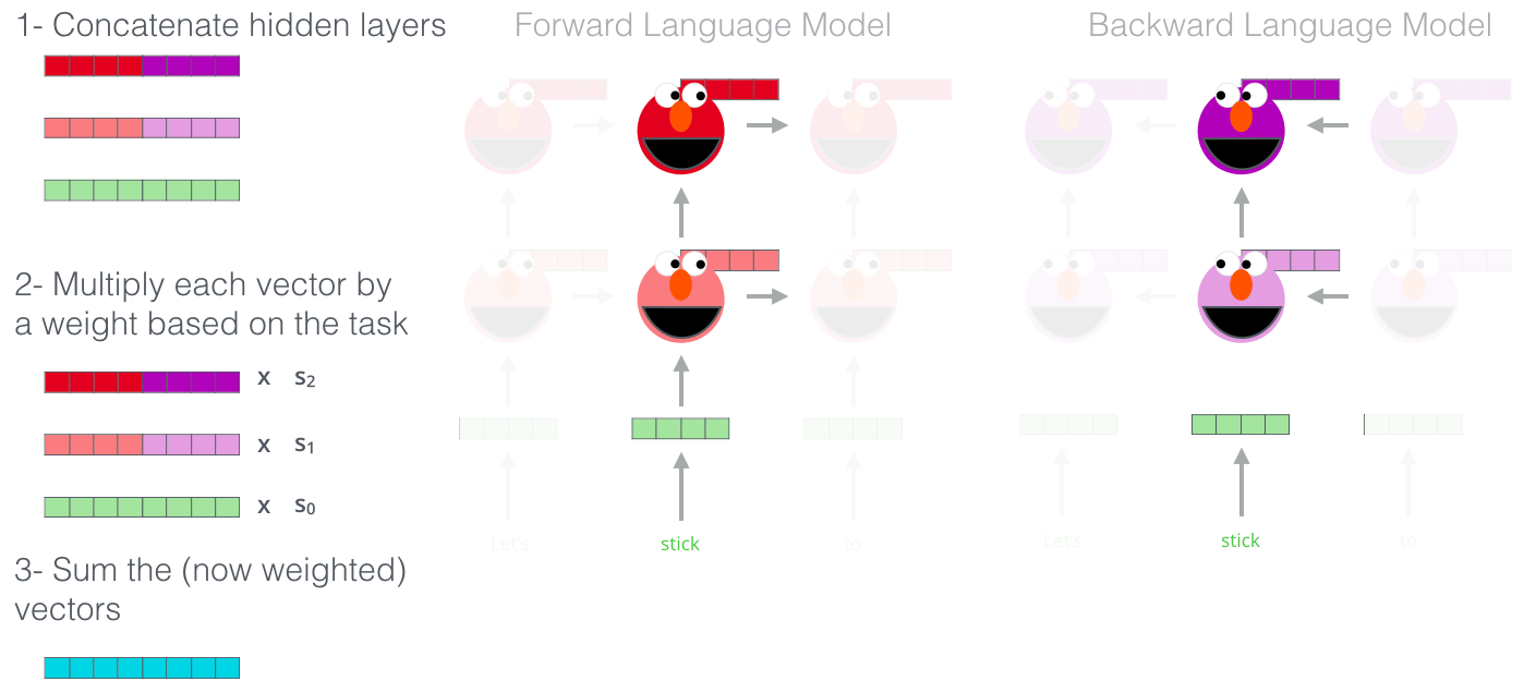
ELMo collapses all alyers in representation set $\mathbf{R}$ into a single vector $\mathbf{ELMo}_k = E(R_k; \Theta_e)$.

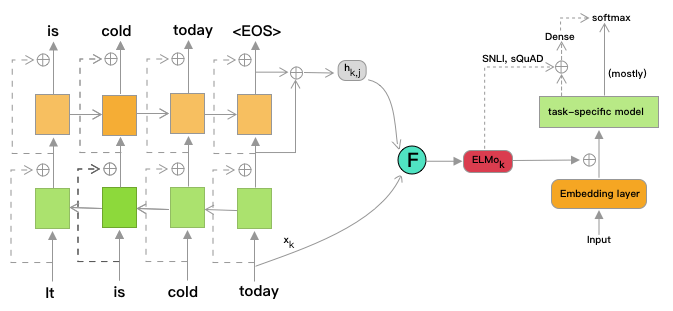
Here previous work like TagLM^[17], CoVe^[18] just selects the top layer.

ELMo computes a task-specific weighting of all BiLM layer representations:

$$ELMo_{o_k}^{task} = E(R_k ; \Theta^{task}) = \gamma^{task} \sum_{j=0}^L s_j^{task} \mathbf{h}_{k,j}^{LM}$$

where s_{task} are softmax-normalized weight, and scalar param $y^{task}$ allows the task model to scale the entire ELMo vector.

ELMo embedding^[23]

How to utilize ELMo into downstream supervised tasks?

Given:

• pretrained biLM with residual conection between LSTM layers
• a supervised task-specific model

Let $\mathbf{x}_k$ denote context-independent token representation (traditional embedding, like w2v, or compositional char cnn embeddings)

How to use EMLo?

• Freeze the biLM weights, run the biLM, and record all the layer representations for each word;
• End task model learn previous linear weights $s^{task}$
  • Usage: concat ELMo vector $\mathbf{ELMo}_k^{task}$ with $\mathbf{x}_k$, and feed concatenated $ [\mathbf{x}_k, \mathbf{ELMo}_k^{task}] $ into the task-specific model.
  • Partially empirically practical on SNLI, SQuAD, replace the output $\mathbf{h}_k$ with $ [\mathbf{h}_k, \mathbf{ELMo}_k^{task}]$, followed by one more domain-specific linear layer.

Fine-tuning pretraining

OpenAI Transformer GPT (generative pre-training)

Problems: NLP with NN suffers from a dearth of annotated resources.

model:

• Left-To-Right google Transformer^[20]
• Use BPE vocabulary^[21]
• Activation function: Gaussian Error Linear Unit (GELU) ^[22]

Two stage:
1) Unsupervised training on unannotated data with LM objective

• Aim: find a good initialization point.
• LM objective: $$L_1 (U) = \sum_i \log P(u_i \vert u_{i-k},...,u_{i-1};\Theta)$$ where k is the context window size
• LM model: a multi-headed self-attention operation over the input context tokens followed by position-wise feedforward layers: $$h_0 = UW_e + W_p$$ $$h_l = \text{transformer block}(h_{l-1}) \quad \forall \quad i \in [1,n])$$ $$P(u) = \text{softmax} (h_nW_e^T)$$ where $U= (u_{-k},...,u_{-1})$ is the context vector of tokens, n is the # of layers, $W_e$ is the token embedding matrix, and $W_p$ is the position embedding matrix.

2) Supervised training on target tasks

Given a labeled dataset C of input tokens $x^1,...,x^m$ along with a label y, and pretrained LM.

Feed the input through our pretrained LM to get the final transformer block’s activation $h_l^m$. Then pass them to an added linear output layer with parameter $W_y$ to predict y:

$$P(y|x^1,...,x^m) = \text{softmax} (h_l^m W_y)$$

The objective is:

$$L_2 (C) = \sum_{x,y} \log P(y \vert x^1,...,x^m)$$

Found including LM as an auxiliary objective can improve generalization of supervised model and accelerate convergence. Hence, the objective is:

$$L_3(C) = L_2(C) + \lambda \times L_1(C)$$

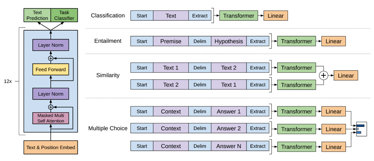
As the figure shows, Transformer GPT model could be applied in different discriminative NLP tasks. For tasks that contains more than 1 sentence, a delimiter token ($) is added in between.

• Classification: directly feed text
• RTE: concat premise $p$ and hypothesis $h$ with a delimiter token(dollar) in between: [p; $ ; h]
• Similarity: no inherent ordering between sentences. We concat both possible sentence orderings (with a delimiter token $ in between)
• QA and Commonsense Reasoning: given context document $z$, a question $q$, and a set of possible answer $a_k$, concatenate the document context and question with each possible answer, adding delimiter in between: $[z;q;\$;a_k]$.

BERT (Google 2018)

BERT: Bidirectional Encoder Representations from Transformers

• Model architecture: multi-layer bi-directional Transformer encoder
• Activation functions: GElu (same as OpenAI GPT)
• Most important improvements: MLM pretraining!

BERT’s pretraining on 2 tasks

Task#1: Masked LM (MLM)

Masked 15% of the input tokens at random, and predicting masked tokens.

Potential problems:

1. Masked tokens are never seen, leading to mismatch between pretraining and fine-tuning.
   Solution: 80% of the time, replace the word with [MASK] token; 10% with random words; the rest 10% unchanged (to bias the representation towards actual observed word).
2. Masking 15% tokens requires more convergence time in pretraining steps.
   Solution: it deserves compare with empirical improvements.

Task#2: Next Sentence Prediction

Task: binarized next sentence prediction (in order to handle relationships between multiple sentences)

• Downstream tasks like QA and NLI requires understanding the relationship between two ajacent sentences. Specifically, predicting whether sentence A is followed by B or not.

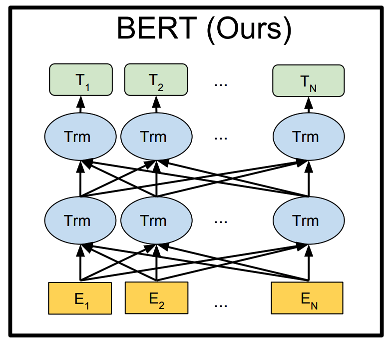
How to employ BERT on downstream tasks?

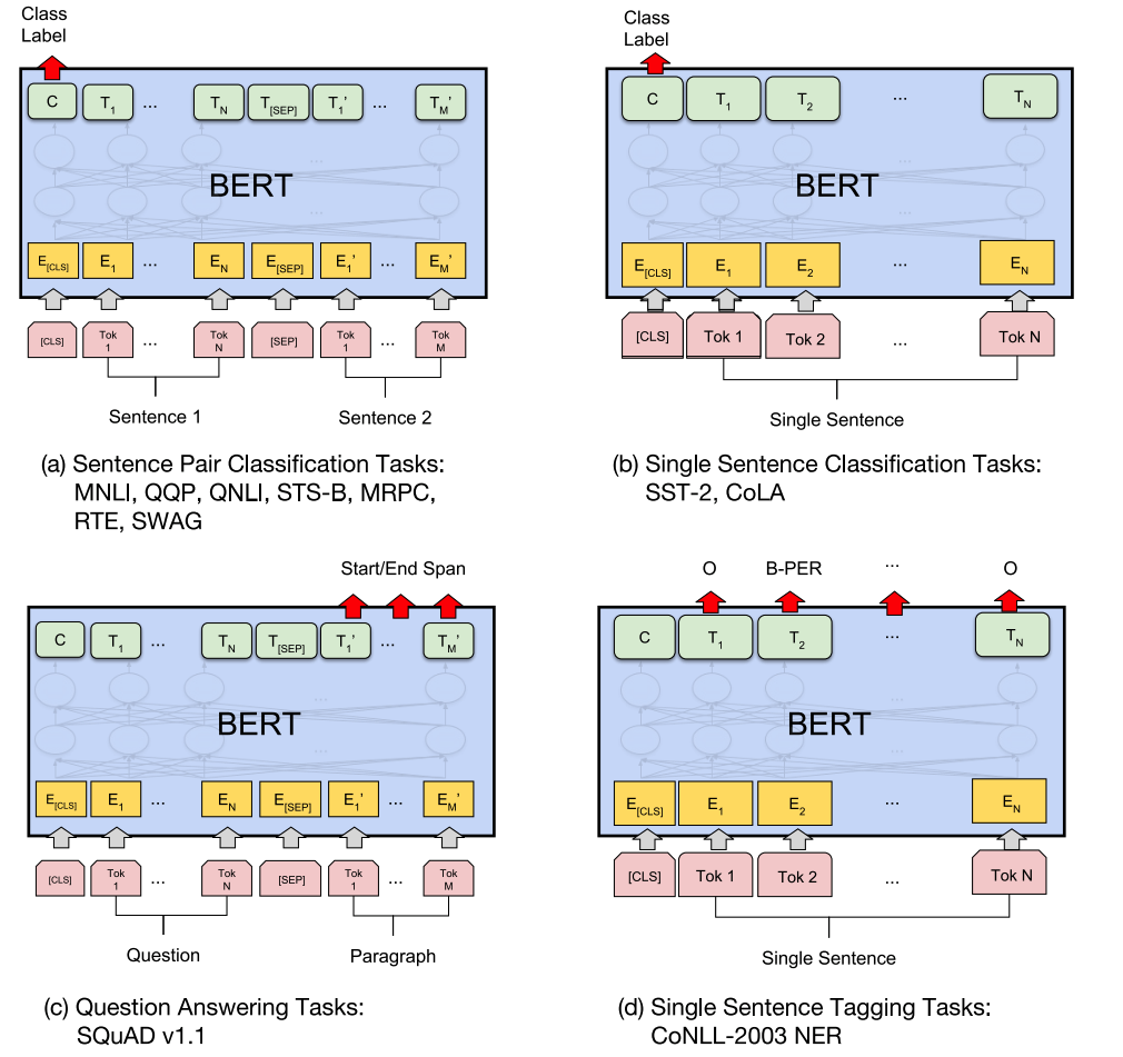
In above figure, $E$ represents the input embedding, $T_i$ represents the contextual representation of token i, [CLS] is the special symbol for classification output, and [SEP] is the special symbol to separate non-consecutive token sequences.

• For sequence-level classification tasks, take the final hidden state (i.e. the Transformer output) for the first token in the input. Feed it into a classification FFNN followed by a softmax.
• For span-level or token-level prediction tasks, as shown in the figure.
• BERT + FFNN + softmax

Bert as a feature extractor

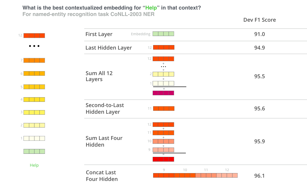
Like ELMo as a feature-based approach, use pretrained BERT to create ELMo-like contextualized word embeddings, and feed them to a domain-specific model.

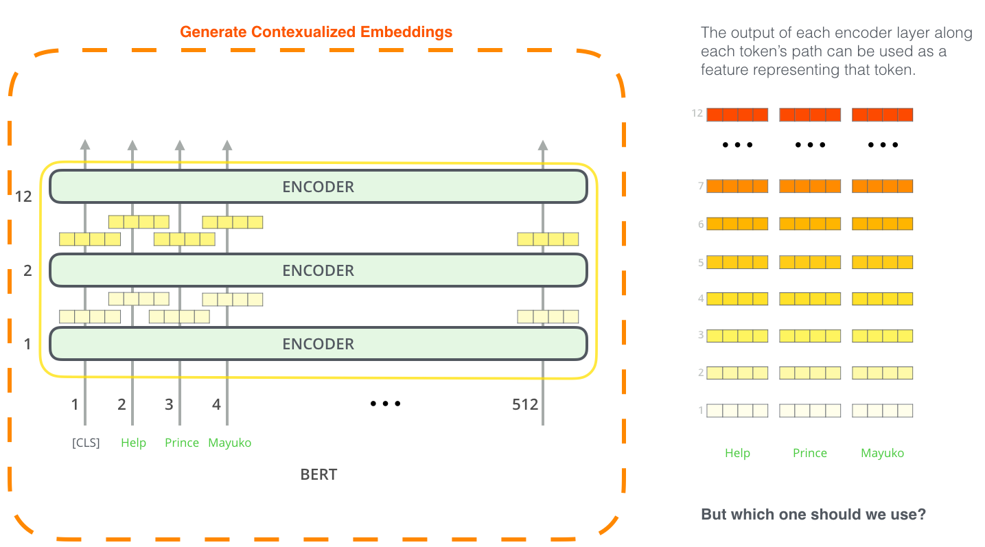
Concating the token representations from the top 4 hidden layers of pretrained Transformer, is only 0.3 F1 behind the fine-tuning BERT. It can be seen that BERT is effective for both the finetuning and feature based approaches.

Bert example^[23]

Future work

Investigate the linguitic phonomena that may or may not be captured by BERT.

Comparison between ELMo, OpenAI GPT and BERT

Model	architecture	pretraining task	Usage style
ELMo	bi-LSTM	LM	feature-based
OpenAI GPT	left-to-right Transformer	LM	fine-tuning
BERT	bi-Transformer	MLM, NSP	fine-tuning

Training time: Transformer < ConvNets < Simple RNNs < LSTMs .

References

---

1. 1.Bengio, Y., Ducharme, R., Vincent, P., & Jauvin, C. (2003). A neural probabilistic language model. Journal of machine learning research, 3(Feb), 1137-1155. ↩
2. 2.R. Miikkulainen and M.G. Dyer. Natural language processing with modular neural networks and distributed lexicon. Cognitive Science, 15:343–399, 1991. ↩
3. 3.What’s the difference between distributed and distributional (semantic) representations? Quora. Retrieved January 7, 2019 ↩
4. 4.Zellig Harris. 1954. Distributional structure. Word, 10(23):146–162. ↩
5. 5.Mikolov, T., Chen, K., Corrado, G., & Dean, J. (2013). Efficient estimation of word representations in vector space. arXiv preprint arXiv:1301.3781. ↩
6. 6.Mikolov, T., Sutskever, I., Chen, K., Corrado, G. S., & Dean, J. (2013). Distributed representations of words and phrases and their compositionality. In Advances in neural information processing systems (pp. 3111-3119). ↩
7. 7.Bojanowski, P., Grave, E., Joulin, A. & Mikolov, T. (2017). Enriching Word Vectors with Subword Information. Transactions of the Association for Computational Linguistics, 5, 135--146. ↩
8. 8.Pennington, J., Socher, R. & Manning, C. D. (2014). Glove: Global Vectors for Word Representation. EMNLP 2014. ↩
9. 9.Weng L. (2017, Oct 15). Learning Word Embedding [Blog post]. Retrieved from https://lilianweng.github.io/lil-log/2017/10/15/learning-word-embedding.html ↩
10. 10.Ruder S. (2018, Jul 08) NLP's ImageNet moment has arrived [Blog post]. Retrieved from https://thegradient.pub/nlp-imagenet/ ↩
11. 11.Peters, M. E., Neumann, M., Iyyer, M., Gardner, M., Clark, C., Lee, K., & Zettlemoyer, L. (2018). Deep contextualized word representations. arXiv preprint arXiv:1802.05365. ↩
12. 12.Howard, J., & Ruder, S. (2018). Universal language model fine-tuning for text classification. In Proceedings of the 56th Annual Meeting of the Association for Computational Linguistics (Volume 1: Long Papers) (Vol. 1, pp. 328-339). ↩
13. 13.Radford, A., Narasimhan, K., Salimans, T., & Sutskever, I. (2018). Improving language understanding by generative pre-training. ↩
14. 14.Devlin, J., Chang, M. W., Lee, K., & Toutanova, K. (2018). Bert: Pre-training of deep bidirectional transformers for language understanding. arXiv preprint arXiv:1810.04805. ↩
15. 15.Wieting, J., Bansal, M., Gimpel, K., & Livescu, K. (2016). Charagram: Embedding words and sentences via character n-grams. arXiv preprint arXiv:1607.02789. ↩
16. 16.Neelakantan, A., Shankar, J., Passos, A., & McCallum, A. (2015). Efficient non-parametric estimation of multiple embeddings per word in vector space. arXiv preprint arXiv:1504.06654. ↩
17. 17.Peters, M. E., Ammar, W., Bhagavatula, C., & Power, R. (2017). Semi-supervised sequence tagging with bidirectional language models. arXiv preprint arXiv:1705.00108. ↩
18. 18.Bryan McCann, James Bradbury, Caiming Xiong, and Richard Socher. 2017. Learned in translation: Contextualized word vectors. In NIPS 2017. ↩
19. 19.Stephen Merity, Nitish Shirish Keskar, and Richard Socher. 2017a. Regularizing and Optimizing LSTM Language Models. arXiv preprint arXiv:1708.02182 . ↩
20. 20.Vaswani, A., Shazeer, N., Parmar, N., Uszkoreit, J., Jones, L., Gomez, A. N., ... & Polosukhin, I. (2017). Attention is all you need. In Advances in Neural Information Processing Systems (pp. 5998-6008). ↩
21. 21.R. Sennrich, B. Haddow, and A. Birch. Neural machine translation of rare words with subword units. arXiv preprint arXiv:1508.07909, 2015. ↩
22. 22.D. Hendrycks and K. Gimpel. Bridging nonlinearities and stochastic regularizers with gaussian error linear units. arXiv preprint arXiv:1606.08415, 2016. ↩
23. 23.Alammar J. (2018, Dec 3). The Illustrated BERT, ELMo, and co. (How NLP Cracked Transfer Learning) [Blog post]. Retrieved from https://jalammar.github.io/illustrated-bert/ ↩
24. 24.Towards data science: FROM Pre-trained Word Embeddings TO Pre-trained Language Models — Focus on BERT ↩