Name Entity Recognition (NER) labels sequences of words in a text which are the names of things, such as person and company names, or gene and protein names.
Approaches:
- Statistical ML methods: HMM, MEMM, CRF
- Deep learning methods: RNN-CRF, CNN-CRF
Hidden Markov Model

HMM consists of a discrete-time, discrete-state Markov chain, with hidden states $z_t \in {1,…,K} $
, plus an observation model $p(\mathbf{x}_t|z_t)$.
HMM is a generative model that optimises the likelihood $P(W|T)$, consisting of three components:
- Initial probability $\pmb{\pi}$
- Transition probability matrix $\pmb{A}$
- Emission probability matrix $\pmb{B}$.
The joint distribution is:
We estimate the posterior by combining the likelihood and the prior P(T).
HMM states only conditions on the previous state.
HMM cons: Independence assumptions.
Maximum-Entropy Markov Model (MEMM)
HMM based on the probabilities of transmission probability matrix and emission probability matrix. It is hard to encode the knowledge into these two matrices. If we include many knowledge sources, like capitalisation, the presence of hyphens, word endings. It is not easy to fit the probability like $P(\textrm{capitalisation} | \textrm{tag}), P(\textrm{hyphen} | \textrm{tag}), P(\textrm{suffix} | \textrm{tag}), P(\textrm{suffix} | \textrm{tag})$ into an HMM-style model.
HMM assumes the independence between observations $z$, while MEMM does not. However, MEMM suffers from the label bias problem.

MEMM is a discriminative model. It computes the posterior $P(Z=T|X=W)$ directly. MEMM states conditioned on the previous state and current observation.
where $f{\cdot}$ is real-valued feature functions, $Z$ is a normalization term.
Thus,
Decoding: Viterbi algorithm.
Pros over HMM: offer increased freedom in choosing features to represent obervations.
Strict left-to-right word classifier.- Cons: only use left sequence information. It cannot consider future sequence information.
MEMM weakness:
- Label bias problem: states with low-entropy transition distributions “effectively ignore their observations”. MEMM normalizes over the set of possible output labels at each time step, which is locally normalized. “Conservation of score mass just says that the outgoing scores from a state for a given observation are normalized.”[7] The result is any inference process will bias towards states with fewer outgoing transitions.
CRFs were designed to overcome this weakness.
vs HMM
unlike the HMM, the MEMM can condition on any useful feature of the input observation. In the HMM this wasn’t possible because the HMM is likelihood-based, hence would have needed to compute the likelihood of each feature of the observation.
$Y$ denotes the state sequence, $X$ denotes the observation.
HMM
MEMM
To estimate the individual probability of a transition from a state $q’$ to a state $q$ producing an observation $o$, build a MaxEnt model:
CRF
Linear-Chain CRF
Modeling the distribution of a set of ouputs $y_{1:T}$ given an input vector $\mathbf{x}$.
where $\lambda$ are the free parameters of the potentials, common form:
where are features.
Thus,
Given a set of input-output sequence pairs, . We can learn the parameters $\lambda$ by Maximum Likelihood. Under the i.i.d. data assumption, the log likelihood is:
Cons: heavily rely on engineering features
BiLSTM-CRF
Intuition:
Capture both information from history (forward LSTM) and future (backward LSTM) using bi-LSTM; Also use sentence level tag information (after concatenation of both forward and backward LSTM/GRU hidden states in each time step) followed by the CRF model; Each output after concatenation can be regarded as a sentence level output.[2] CRF can help learn the boundary constraints, for example, ‘B-‘ is the start of a tag.
Pros: More robust, less affected by the removal of engineering features
Cons: RNNs are not as GPU-efficient as CNNs in terms of training speed and efficiency.
Let $y$ be the tag sequence and $x$ an input word sequence. Then, we have
where
In BiLSTM-CRFs, two potentials: emission and transition. The emission potential for the word $i$ comes from the hidden state of the BiLSTM at timestep $i$. The transition scores are stored at $\mathbf{P} \in \mathbb{R}^{|T| \times |T|}$. In the following implementation[8], $\mathbf{P}_{y_i, y_i-1}$ is the score of transitioning to tag $i-1$ from tag $i-1$.

1 | import torch |
Stack-LSTM
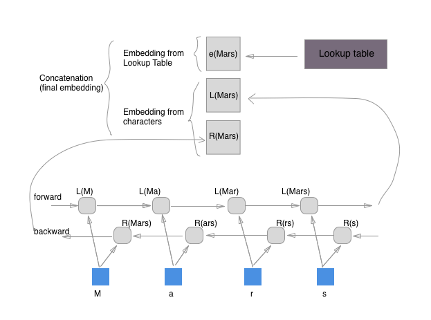
Char-based word representation indicates the word internal information, whilst pretrained word embeddings hold contextual text information.
Then, concat character-based word representation using Bi-LSTM and pretrained word embeddings as the final embeddings. [6]
ID-CNN-CRF
Pros: fast, resource-efficient
Dilation convolutions:
- context does not need to be consecutive
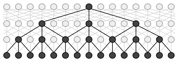
By stacking layers of dilated convolutions of exponentially dilation width, we can expand the size of the effective input width to cover the entire length of most sequences using only a few layers: the size of the effective input width for a token at layer l is now given by 2l+1-1
- Let xt denotes the token in timestep t, Wt is a sliding window of width $r$ tokens on either side of each token in the sequence, the conventional convolution output output ct is:
, where $\bigoplus$ is vector concatenation. - Dilated convolution is defined over a wider effective input width by skpping over \delta inputs, where $\delta$ is the dilation width. The dialated convolution is:
When $\delta$ is 1, dialated convolution is equivalent to a simple convolution.
Model: Stacked dilated CNNs [3]
Let the dilated Conv layer of dilation width $\delta$ as , layers output:
And add a final dilation-1 layer to the stack:
Finally, apply the simple affine transformation $W_0$ to the final representation for each token :
ID-CNNs generate token-wise representation (corresponding to logits for each token in RNNs) for each token.
In comparison with BiLSTM-CRF
Bi-LSTM or ID-CNNs calculates the logits for each token, whilst CRF layer capture the transmission probability of sequential inputs, i.e. use NNs to predict each token’s label independently, or apply Viterbi inference in a chain structured graphical model.
BERT
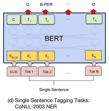
Bidirectional Transformer for Language model, with pretraining methods of Masked Language Models (predicting randomly masked 15% tokens of each sentence) and next sentence prediction (to capture information of ajacent sentences).[5]
Chinese NER
Chinese NER
Word-based approach
- Intuitive pipeline: segmentation → NER
- Suffer from segmentation error: NE imports OOV errors in segmentation, and incorrectly segmented entity boundaries lead to NER errors.
Char-based approach
- Char-based NER outperform word-based approach in Chinese NER.
- Cons: Explicit word and word sequence information are not fully exploited.
Solution:
- Lattice LSTM: leverage both char sequence and lexicon word information.
- FLAT
Char-based LSTM-CRF model
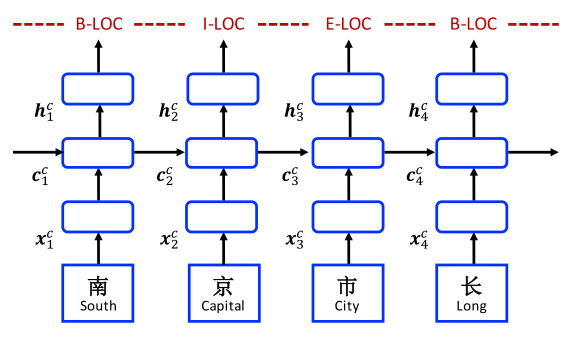
$\mathbf{x}_j^c = \mathbf{e}^c(c_j)$, where $\mathbf{e}^c$ denotes a char embedding lookup table.
Bi-LSTM output: $\mathbf{h_j^c} = [\overrightarrow{\mathbf{h}_j^c} ; \overleftarrow{\mathbf{h}_j^c}]$
CRF model use $\mathbf{h_1^c}, \mathbf{h_2^c}, …,\mathbf{h_m^c}$ for sequence labelling.
Char + bi-char
Concat char embeddings with char-bigram embeddings.
,where $\mathbf{e}^b$ denotes a char bigram lookup table
Char + softword
- add segmentation as soft features by concatenating segmentation label embedding to char embeddings
, where $\mathbf{e^s}$ signals the segmentation label on the char $c_j$ given by a word segmentor with BMES scheme.
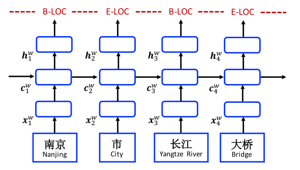
Word-based model
The input for each word $w_i$: $\mathbf{x_i^w} = \mathbf{e}^w (w_i)$, where $e^w$ denotes the word embedding lookup table.
Then feed word embeddings into bi-directional LSTMs.
Integrating char-representations
concat char-based word representation $\mathbf{x}_i^c$ (from cahr-LSTMs or char-CNNs) with pretrained word embeddings $\mathbf{e}^w(w_i)$: $\mathbf{x}_i^w = [\mathbf{e}^w(w_i); \mathbf{x}_i^c]$
1.Word + char bi-LSTMs: bi-LSTMs with chars as input in each time step.
2.Word + char-uni-LSTM
3.Word + char-CNNs
Use char sequence of each word to obtain its char representation $\mathbf{x}_i^c$:
, where $ k=3 $ is the kernel size and $max$ denotes the max-pooling.
Lattice LSTM
Let $s$ denotes input sequence.
- Char-level: , where denotes the character.
- Word-level: , where denotes the token in the word sequence.
In comparison with char-based model:
Char embedding: $\mathbf{x}_j^c = \mathbf{e}^c(c_j)$
Basic recurrent LSTM:
where $\mathbf{i}^c_j$, $\mathbf{f}^c_j$, $\mathbf{o}^c_j$ denotes a set of input, forget and output gates, respectively. $\mathbf{c}^c_j$ denotes the char cell vector, $\mathbf{h}^c_j$ denotes the hidden vector on each char $c_j$, $\mathbf{W}^{c^T}$, $\mathbf{b}^c$ are parameters.
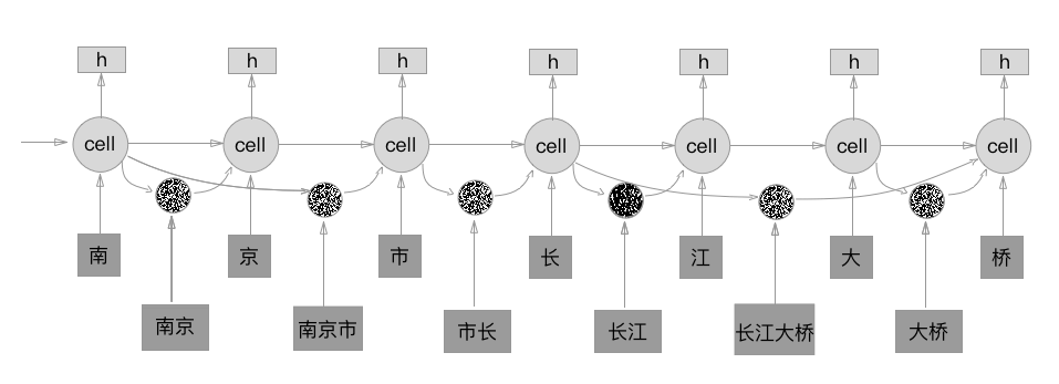
The computation of cell vector considers lexicon subsequence in the sentence[4].
Each subsequence is:
, where $\mathbf{e}^w$ denotes the word embedding lookup table.
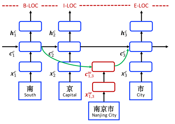
The word cell represents the recurrent state of from the beginning of the sentence. The is:
where , are input and forget gates. There is no output gate for word cells since labelling is performed only at the char level.
Here as an additional recurrent path for information flow for each . It applies an additional gate for each subsequence cell for controlling its contribution into :
Then cell vector is:
where the gate value , are normalised to and by setting the sum to 1:
CRF decoding
On top of , , …, , where $\tau$ is $n$ for char-based and lattice-based models and $m$ for word-based models. The probability of a label sequence is:
where $y’$ denotes an arbitrary label sequence, is a model parameter specific to and is a bias specific to and .
Sentence-level log-likelihood loss with L2 regularization:
where $\lambda$ is the $L_2$ regularisation parameter and $\Theta$ represents the parameter set.
FLAT
Flat-Lattice Transformer (FLAT)
References
- 1.Jurafsky, D., & Martin, J. H. (2014). Speech and language processing (Vol. 3). London: Pearson. ↩
- 2.Huang, Z., Xu, W., & Yu, K. (2015). Bidirectional LSTM-CRF Models for Sequence Tagging. arXiv preprint arXiv:1508.01991. ↩
- 3.Strubell, E., Verga, P., Belanger, D., & McCallum, A. (2017). Fast and accurate entity recognition with iterated dilated convolutions. arXiv preprint arXiv:1702.02098. ↩
- 4.Zhang, Y., & Yang, J. (2018). Chinese NER Using Lattice LSTM. arXiv preprint arXiv:1805.02023. ↩
- 5.Devlin, J., Chang, M. W., Lee, K., & Toutanova, K. (2018). BERT: Pre-training of Deep Bidirectional Transformers for Language Understanding. arXiv preprint arXiv:1810.04805. ↩
- 6.Lample, G., Ballesteros, M., Subramanian, S., Kawakami, K., & Dyer, C. (2016). Neural Architectures for Named Entity Recognition. arXiv preprint arXiv:1603.01360. ↩
- 7.The Label Bias Problem ↩
- 8.PyTorch BiLSTM-CRF ↩
- 9.BiLSTM-CRF Explanation (in Chinese) ↩
