A note for NLP Interview.
Statistical ML
LR vs SVM
Difference:
- LR uses logistic loss, while SVM uses hinge loss.
- LR is sensitive to outliers, while SVM is not.
- SVM is suitable for small training set, while LR needs much.
- LR tries to find a hyperplane that stays far away with all points (all points count), whereas SVM only aims at keeping away support vectors.
- LR requires feature enginnering, SVM uses kernel trick.
- SVM is non-parametric methods, whereas LR is parametric model.
Logistic Regression (LR)
Logistic Regression (LR) is a linear mapping from features $x$ to labels $y \in \{ 0,1 \}$ with sigmoid function $g(z)=1/(1+\exp(-z))$.
The LR is fomulated as:
The derivative of sigmoid function is:
LR can be used for binary classification, thus
That is,
Given the training data, the features $x = \{ x_1, x_2, \cdots, x_m \}$ and labels $y = \{ y_1, y_2, \cdots, y_m \}$. The maximum likelihood function is:
With gradient ascend algorithm, we have $\theta : \theta + \alpha \nabla_{\theta}\ell (\theta)$.
If we only use one sample to train, the update can be formulated as:
The loss function is:
Linear SVM
Given a training dataset of $m$ points of the form $(\mathbf{x}_1,y_1), \cdots,(\mathbf{x}_m,y_m)$, where $y \in \{-1,1\}$, each indicating the calss to which the point $x_i$ belongs. We want to find the maximum-margin hyperplane that divides the group of points $\mathbf{x}_i$ into two groups so that the distance between the hyperplane and the nearest point from either group is maximized.
Any hyperplane can be written as the set of points $\mathbf{x}$ satisfying $\mathbf{w}^T\mathbf{x}+\mathbf{b}=0$.
Hard margin
If the training data is linearly separable, we can select to parallel hyperplanes that separate the two clases of data, so that the distance between them is as large as possible. The region bounded by these two hyperplanes is called the “margin”, and the maximum-margin hyperplanes is the hyperplane that lies halfway between them.
The optimization aims to “minimize $\Vert \mathbf{w} \Vert$ subject to $y_i (w^T x_i + b) \geq 1$ for $\forall i$”:
- Maximize the margin: $ \min_{\mathbf{w,b}} \frac{1}{2} \Vert \mathbf{w} \Vert^2$
- Classify: $y_i (w^T x_i + b) \geq 1, \quad i=1,2,3,\cdots,m$
where the $\mathbf{w},\mathbf{b}$ determine our classifier $\mathbf{x} \rightarrow \textrm{sign} (\mathbf{w}^T \mathbf{x} + \mathbf{b})$
Soft margin
Hinge Loss
When the data are not linearly separable, the hinge loss[1] is helpful:The hinge loss is zero if the constraint $y_i (w^T x_i + b) \geq 1$ is satisfied, i.e., if $\mathbf{x}_i$ lies on the correct side of the margin. For data on the wrong side of the margin (-1 vs 1), the hinge loss is proportional to the distance from the margin.
Soft margin objective
The optimization goal is to minimizewhere the parameter $\lambda$ determines the trade-off between increasing the margin size and ensuring that the $\mathbf{x}_i$ lie on the correct side of the margin. Thus, for sufficiently small values of $\lambda$, the second term in the loss function will become negligible, hence it will behave similar to the hard-margin SVM.
CRF
Loss
Let $x$ represent the observation, $y$ denote the labels. CRF can be formulated as:
where
The loss function would be given as:
Decision Tree
GBDT / Xgboost
L1/L2 Regularization
L1 regularization
The L1 regularization is given as:
Thus,
The weight update is:
L2 regularization
The L2 regularization is given as:
Thus,
The weight update is:
Implementation
KMeans
KNN
Class Imbalance / Long-tailed Learning
Extant class imbalance[12][13] methods:
- the input to a model (Data modification)
- Under-sampling
- Over-sampling
- Feature Transfer
- the output of a model (Post-hoc correction of the decision threshold)
- Modify threshold
- Normalize weights
- the internals of a model (e.g., loss function)
- Loss balancing
- Volume weighting
- Average top-k loss
- Domain adaptation
- Label aware margin
Information Theory
KL Divergence
Kullback-Leibler (KL) divergence[9] (a.k.a, relative entropy) is a measure of how one probability distribution is different from a second, reference probability distribution.
Consider two probability distributions $P$ and $Q$. Usually, $P$ represents the data, the observations, or a measured probability distribution. Distribution $Q$ represents instead a theory, a model, a description or an approxmation of $P$. The KL divergence is then interpreted as the average difference of the number of bits required for encoding samples of $P$ using a code optimized for $Q$ rather than one optimized for $P$.
For discrete probability distributions $P$ and $Q$ defined on the same probability space $\chi$, the relative entropy from $Q$ to $P$ is defined to be:
The relative entropy can be interpreted as the expected message-length per datum that must be communicated if a code that is optimal for a given (wrong) distribution $Q$ is used, compared to using a code based on the true distribution $P$.
where $\mathbb{H}(P \vert Q)$ indicates the cross entropy of P and Q, $\mathbb{H}(P)$ is the entropy of P.
Properties
- Non-negative
- Asymmetric
JS Divergence
Jensen-Shannon (JS) divergence is a measure of similarity between two probablity distributions.
where $M = \frac{1}{2}(P+Q)$
Properties
- Symmetric
- Bound $0 \leq JSD \leq 1$
Mutual Information
Mutual Information (MI)[10] measures the mutual dependence between the two variables.
For discrete variables $X$ and $Y$ the MI is:
Properties
- Non-negative: $I(X;Y) \geq 0$
- Symmetry: $I(X;Y) = I(Y;X)$
Evaluation Metric
ROC / AUC
ROC
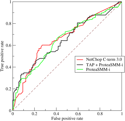
Reiceiver Operating Characteristic (ROC) Curve is a plot that illustrates the diagnostic ability of a binary classifier system as its discrimination threshold is varied.
- x-axis: false positive rate (FPR), a.k.a, sensitivity, recall, probability of detection.
- y-axis: true positive rate (TPR), a.k.a. probability of false alarm.
ROC is a comparison of two operating characteristics (TPR and FPR) as the criterion changes.
True Positive Rate (TPR) is a synonym for recall and is therefore defined as follows:
False Positive Rate (FPR) is defined as follows:
An ROC curve plots TPR vs. FPR at different classification thresholds. Lowering the classification threshold classifies more items as positive, thus increasing both False Positives and True Positives.

AUC
Area under the ROC Curve (AUC) provides an aggregate measure of performance across all possible classification thresholds. A model whose predictions are 100% wrong has an AUC of 0.0; one whose predictions are 100% correct has an AUC of 1.0.

1 | import numpy as np |
F1-Measure
- Micro-F1: calculate metrics globally by counting total TP,FN,FP
- Macro-F1: calculate metrics for each label => unweighted mean.
- Weighted-F1: calculate metrics for each label => average weighted by support (# of true instances for each class)
Comparison between ROC and F1-measure:
- Both look at the precision scores (TPR): ROC looks at the True Positive Rate (TPR/Recall) and False Positive Rate (FPR) while F1 looks at Positive Predictive Value (PPV/Precision) and True Positive Rate (TPR/Recall).[11]
- F1 score cares more about the positive class, such as highly imbalanced dataset where the fraction of positive class is small.
- ROC cares equally about the positive and negative class or the dataset is quite balanced.
Deep Learning
Batch Norm vs Layer Norm
- BN normalizes along one batch (first dim), LN does on one sample (last dim).
- Refer to details
Gradient Vanishing/Exploding
Gradient vanishing/exploding arises from the issues of backpropagation, in other words, the accumulated multiplication of smaller-than-1 or greater-than-1 gradient values.
Solution
- Pretraining-Finetuning per layer
- Gradient Clip / Weight Regularization
- Activation function: avoid to use sigmoid.
- Appropriate weight initialization: Xavier-Glorot initialization[4]
- Batch Norm: reduce the covariant shift of training dataset.
- Residual Connection
- LSTM: refer to [4][5].
RNNs
LSTM
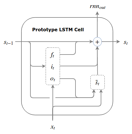
LSTM[6] integrates three gates: input gate, forget gate, and output gate.


GRU
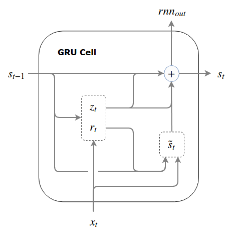
GRU has three gates: update gate (vs input/output gate in LSTM) and reset gate.

Transformer
See Transformer blog
Backprop with Softmax + XE
Refer to [7].
Softmax Forward
Given the softmax written in:
where $a_i, i=1,2,\cdots,N$ is the output logits, $p_i$ is the predicted probability of $i$-th class, and
Computation
The computation of softmax will first reduce the maximum value of $A=[a_1, a_2, \cdots, a_N]$ to avoid the overflow of exp(.).
We have
where $C$ is constant.
Cross Entropy Forward
Denote the Cross Entropy (XE) loss as $H$:
Softmax Derivative
The derivative of softmax w.r.t $a_i$ is:
For brevity, let $\sum = \sum_j^N \exp(a_j)$.
When $i=j$, we have:
When $i \neq j$, we have:
XE+Softmax Derivative
The derivative of XE is:
According to the chain rule, the derivative w.r.t $a_j$ is:
When $i=j$
When $i \neq j$, the Eq. $\eqref{eq:xe_derivative}$ is:
Since above two scenarios are independent, combining Eq. $\eqref{eq:s1}$ and $\eqref{eq:s2}$, we have:
In Eq.$\eqref{eq:one_hot}$, we have $\sum_i^N y_i = 1$;
In Eq.$\eqref{eq:ij}$, we have $\sum_i^N y_i = y_j$.
NLP
Static Word Representation
Word2Vec
Hierarchical Softmax / Negative Sampling
Refer to my blog
- Hierarchical Softmax: $|V| => \log |V|$ using huffman tree
- Negative Sampling
W2V vs GloVe
BPE vs WordPiece
Refer to OOV blog
References
- 1.Wiki: Hinge Loss ↩
- 2.SVM Blog ↩
- 3.SVM Derivatives (in Chinese) ↩
- 4.Written Memories: Understanding, Deriving and Extending the LSTM ↩
- 5.LSTM eased gradient vanishing explanations (in Chinese) ↩
- 6.Understanding LSTM Networks ↩
- 7.Softmax classification with cross-entropy (2/2) ↩
- 8.Softmax+XE Backpropagation (in Chinese) ↩
- 9.Wiki: KL divergence ↩
- 10.Wiki: Mutual Information ↩
- 11.[F1 score vs ROC AUC vs Accuracy vs PR AUC: Which Evaluation Metric Should You Choose?] ↩
- 12.Long-Tail Learning via Logit Adjustment ↩
- 13.Data Imbalance blog ↩
